
While the current advancements in Machine Learning systems’ scoring are indeed impressive, they hit a wall a few years back with respect to their adoption by a broader audience. This has happened because these complex solutions failed to deliver one important human aspect: trust. As their decisions affect people’s lives — from credit consession to self-driving assist systems —, ML must be reliable and trustworthy. As if it weren’t enough, trusting in machines is hard, specially when you are not a specialist or don’t know its inner workings. Remember that many countries today still conduct their public elections using paper-based ballot counting, which although much inefficient, can be verified by any interested citizen (and not only specialists).
For even the simplest environments, many aspects may come into play and create unexpected scenarios were machines behave unreliably. Code bugs, structural fatigue, improper maintance and extreme running conditions are examples of such. In any case, it’s a given that machines operating in such scenarios should always feedback their decisions to the users, describing why they are being taken in order to inform interested parties, maintain logs of its behavior and facilitate troubleshooting.
People should not accept bindly automatic decisions. There’s a great book about this which everyone shoud read: Weapons of Math Destruction, by Cathy O’Neil.
Research on explaining methods for ML has gained traction in the past years. However, intelligent systems have been around for many decates now. So, is this really a new problem? And if not, what’s different?
import numpy as np
import pandas as pd

from sklearn import datasets
from sklearn.datasets import fetch_openml

import matplotlib.pyplot as plt
import seaborn as sns

import IPython.display as display
import PIL.Image

def download_image(url, path):
    r = requests.get(url, allow_redirects=True)
    with open(path, 'wb') as f:
        f.write(r.content)
    return path

def as_image_vector(x):
    x = x.numpy()
    x = x / 2 + .5
    x *= 255

    return np.clip(x, 0, 255).astype('uint8')

def print_predictions(model, x, top=5):
    y = model.predict(x)
    y = tf.nn.softmax(y)
    predictions = decode_predictions(y.numpy(), top)

    for ix, p in enumerate(predictions):
        print(f'Sample {ix}:',
              *(f'  {pred}: {100*prob:.2f}' for _, pred, prob in p),
              sep='\n', end='\n\n')

def plot(y, titles=None, rows=1, i0=0):
    from math import ceil

    for i, image in enumerate(y):
        if image is None:
            plt.subplot(rows, ceil(len(y) / rows), i0+i+1)
            plt.axis('off')
            continue

        t = titles[i] if titles else None
        plt.subplot(rows, ceil(len(y) / rows), i0+i+1, title=t)
        plt.imshow(image)
        plt.axis('off')

def plot_images_and_salency_maps(images, saliency, labels):
    grads_titles = [f'{_p[0][1]} {_p[0][2]:.2%}' for _p in decode_predictions(labels, top=1)]

    plt.figure(figsize=(16, 5))
    plot([*images, *saliency],
        titles=sorted([os.path.splitext(os.path.basename(f))[0] for f in IMAGES])
               + grads_titles,
        rows=2)
    plt.tight_layout()

sns.set_style("whitegrid", {'axes.grid' : False})
Explaining Classic Artificial Intelligence Agents
Most classic artificial intelligence systems — derived from the symbolic approach of AI — were pretty straight forward: they would rely heavily on the ideas of planning and search over a rational optimization space through a sequence of rational actions. For example, path-finding is an important problem for movement optimization systems (used in games, robotics), where one must travel from point A to point B using the least amount of effort (time, steps etc), and can be solved using algorithms like Dijkstra’s or A*.

Similarly, one could “solve” board games such as Othelo or Chess by describing valid states of the environment, the valid moves available and an utility function associated with the probability could. Search algorithms — such as Alpha-Beta Prunning and Monte-Carlo Tree Search — can then be employed to search for the best utility state (and the path that will take us there).

These systems are easy to explain precisely because of the way they were built: they are iterative, rational and direct by nature. If the environment and the actions can be drawn or represented in some form, then we can simply draw the sequence of decisions that comprise the reasioning of the model. In the path-finding example above, we can see exactly which sections of the map are being scanned, until the shortest-path is found between the source the the green dot. As for the MCTS, we can guarantee the solution otimality (with respect to the local search space expanded) by simple inspection.
Explaining Decision-based Models
Classifiers and regression models are agents whose sole action sets consist on giving answers. When explaining such agents, we tend to focus on why some answer was given. So the problem of explaining an answering agent reduces to explaining the answer itself. Consider the toy example problem below:
ds = datasets.load_breast_cancer()

x = pd.DataFrame(ds.data, columns=ds.feature_names)
y = ds.target_names[ds.target]

x.head().round(2)
| mean radius | mean texture | mean perimeter | mean area | mean smoothness | mean compactness | mean concavity | mean concave points | mean symmetry | mean fractal dimension | radius error | texture error | perimeter error | area error | smoothness error | compactness error | concavity error | concave points error | symmetry error | fractal dimension error | worst radius | worst texture | worst perimeter | worst area | worst smoothness | worst compactness | worst concavity | worst concave points | worst symmetry | worst fractal dimension | |
|---|---|---|---|---|---|---|---|---|---|---|---|---|---|---|---|---|---|---|---|---|---|---|---|---|---|---|---|---|---|---|
| 0 | 17.99 | 10.38 | 122.80 | 1001.0 | 0.12 | 0.28 | 0.30 | 0.15 | 0.24 | 0.08 | 1.10 | 0.91 | 8.59 | 153.40 | 0.01 | 0.05 | 0.05 | 0.02 | 0.03 | 0.01 | 25.38 | 17.33 | 184.60 | 2019.0 | 0.16 | 0.67 | 0.71 | 0.27 | 0.46 | 0.12 |
| 1 | 20.57 | 17.77 | 132.90 | 1326.0 | 0.08 | 0.08 | 0.09 | 0.07 | 0.18 | 0.06 | 0.54 | 0.73 | 3.40 | 74.08 | 0.01 | 0.01 | 0.02 | 0.01 | 0.01 | 0.00 | 24.99 | 23.41 | 158.80 | 1956.0 | 0.12 | 0.19 | 0.24 | 0.19 | 0.28 | 0.09 |
| 2 | 19.69 | 21.25 | 130.00 | 1203.0 | 0.11 | 0.16 | 0.20 | 0.13 | 0.21 | 0.06 | 0.75 | 0.79 | 4.58 | 94.03 | 0.01 | 0.04 | 0.04 | 0.02 | 0.02 | 0.00 | 23.57 | 25.53 | 152.50 | 1709.0 | 0.14 | 0.42 | 0.45 | 0.24 | 0.36 | 0.09 |
| 3 | 11.42 | 20.38 | 77.58 | 386.1 | 0.14 | 0.28 | 0.24 | 0.11 | 0.26 | 0.10 | 0.50 | 1.16 | 3.44 | 27.23 | 0.01 | 0.07 | 0.06 | 0.02 | 0.06 | 0.01 | 14.91 | 26.50 | 98.87 | 567.7 | 0.21 | 0.87 | 0.69 | 0.26 | 0.66 | 0.17 |
| 4 | 20.29 | 14.34 | 135.10 | 1297.0 | 0.10 | 0.13 | 0.20 | 0.10 | 0.18 | 0.06 | 0.76 | 0.78 | 5.44 | 94.44 | 0.01 | 0.02 | 0.06 | 0.02 | 0.02 | 0.01 | 22.54 | 16.67 | 152.20 | 1575.0 | 0.14 | 0.20 | 0.40 | 0.16 | 0.24 | 0.08 |
Decision trees are classic answering models that are trivially explained. One can simply draw its decision paths in order to check for irregularities or inconsistencies:
from sklearn.tree import DecisionTreeClassifier
from sklearn.tree import plot_tree

decision_tree = DecisionTreeClassifier().fit(x, y)
def plot_tree_fullscreen(decision_tree):
  plt.figure(figsize=(16, 9))
  annotations = plot_tree(
    decision_tree,
    feature_names=ds.feature_names,
    class_names=ds.target_names,
    filled=True,
    precision=1
  )

  for o in annotations:
    if o.arrow_patch is not None:
      o.arrow_patch.set_edgecolor('black')
      o.arrow_patch.set_linewidth(3)

plot_tree_fullscreen(decision_tree)
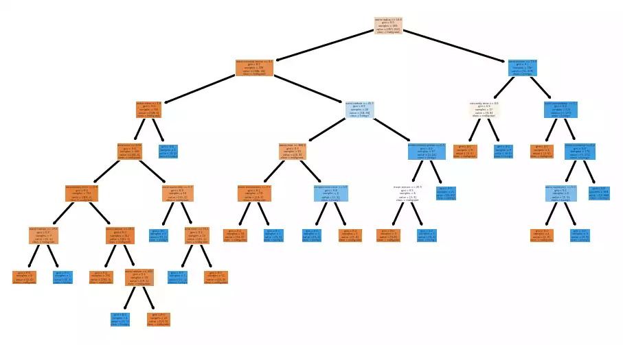
And so are Random Forests, which although much larger and difficult to draw, can be just as easily summarized.
from sklearn.ensemble import RandomForestClassifier
rf = RandomForestClassifier().fit(x, y)

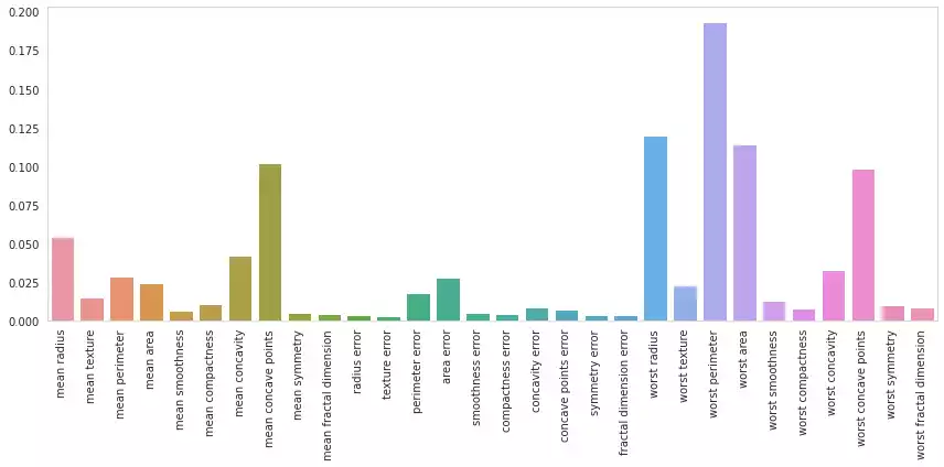
One could check the rate in which each feature appears in the forest’s trees. If a feature’s occurrence is high, then that feature was frequently determinant for the forest’s overall decision process. On the other hand, a feature that rarely appears has less impact in the answer.
def plot_feature_importances(feature_importances):
  plt.figure(figsize=(12, 6))
  sns.barplot(x=ds.feature_names, y=feature_importances)

  plt.xticks(rotation=90)
  plt.tight_layout()

plot_feature_importances(rf.feature_importances_)
Explaining Linear Geometric Models
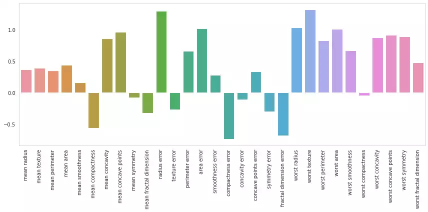
Linear geometric models, such as Linear Regression, Logistic Regression, Linear Support Vector Machines and many others, estimate a variable of interest as a linear combination of the features:
\[p = w\cdot x + b = w_0x_0+w_1x_1+\ldots+w_fx_f + b\]Interpretation is straight forward for this model: s $w_i \to 0$, the variations in feature $i$ becomes less relevant to the overall combination $p$; When $w_i$ assumes a strongly positive value, then feature $i$ positively contributes to the estimation of $p$. Conversely, $w_i$ assuming a negative value implies that feature $i$ negatively contributes to $p$.
As the parameters $w$ are also use to scale the individual features $x$, they are in different scales and cannot be directly compared. This can be remedied by normalizing features into a single scale:
from sklearn.pipeline import make_pipeline
from sklearn.preprocessing import StandardScaler
from sklearn.linear_model import LogisticRegression

p = make_pipeline(
  StandardScaler(),
  LogisticRegression()
).fit(x, y)

lm = p.named_steps['logisticregression']

w, b = lm.coef_, lm.intercept_
plot_feature_importances(w.ravel())
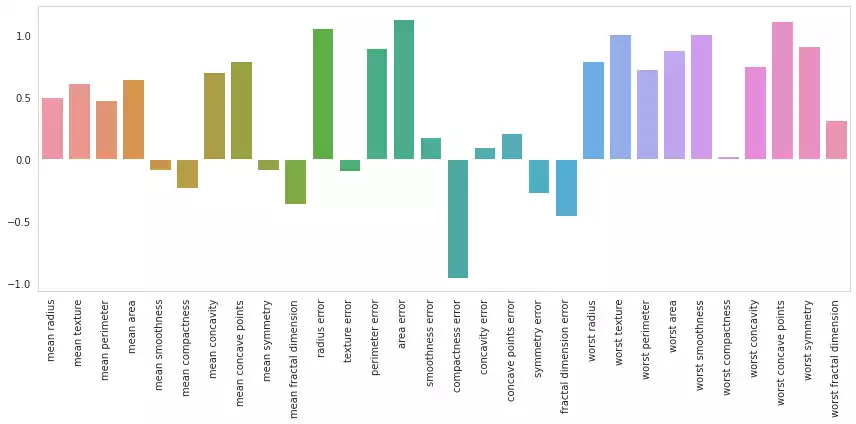
This can also be acomplished when reducing the set with Principal Component Analysis, considering the whole pipeline can be seen as a sequence of matrix multiplications, which is an associative operation:
\[y = (XR)W +b \iff y = X(RW) + b\]from sklearn.decomposition import PCA
lm = make_pipeline(
StandardScaler(),
PCA(n_components=0.99),
LogisticRegression()
).fit(x, y)
w = (lm.named_steps['pca'].components_.T
@ lm.named_steps['logisticregression'].coef_.T)
print(
  f'Original dimensions: {x.shape[1]}',
  f'Reduced dimensions:  {lm.named_steps["pca"].explained_variance_ratio_.shape[0]}',
  f'Energy retained:     {lm.named_steps["pca"].explained_variance_ratio_.sum():.2%}',
  sep='\n'
)

plot_feature_importances(w.ravel())
Original dimensions: 30
Reduced dimensions:  17
Energy retained:     99.11%
Explaining Deep Convolutional Networks
Networks are a very specific sub-set of machine learning. They derive from what’s called the “Connectionist Approach” to artificial intelligence — the idea that intelligence can be achieved by connecting massive amounts of basic processing units through quantitative signals. So their behavior is directly influenced by a complex combination of factors. For modern networks, this is even more convoluted by the successive application of non-linearities across the whole system.
Differently from search algorithms, connectionist models are complicated in nature, which poses higher difficulties in understanding them. Suppose you have a conventional image classification network:
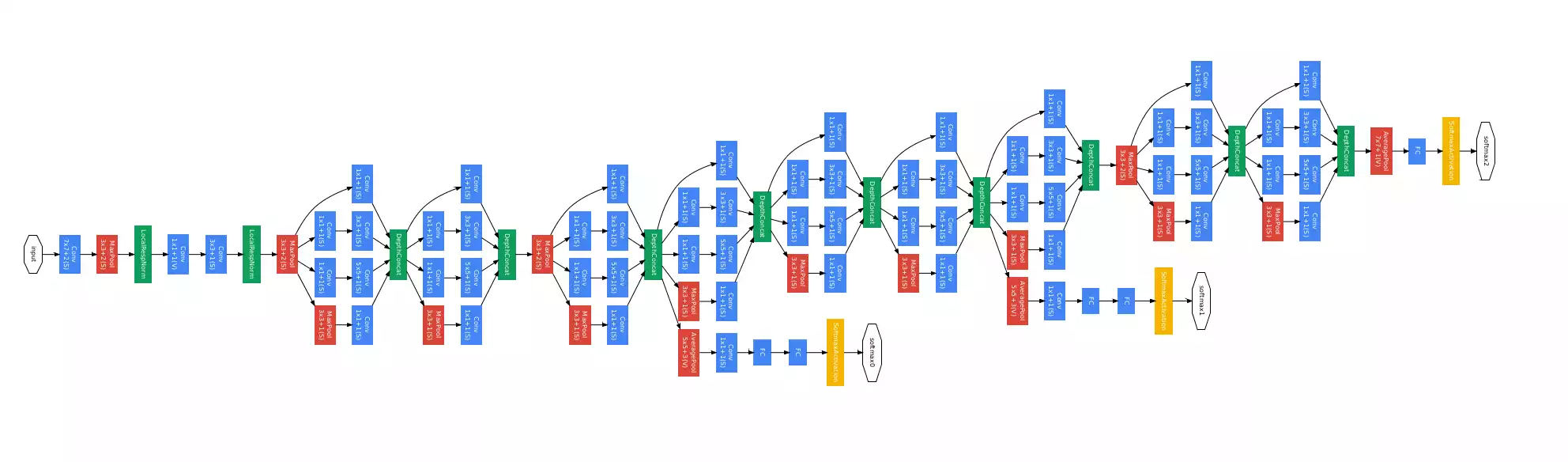
Each blue box represents a set of convolutions between an 3D input signal and multiple kernels and the application of a non-linear function (relu, most likely). Given an input image and the feed-forward signal of that image through the network (the answer), how can one make sense of the answer?
Many solutions were studied over the last years. Some of them involved patching-out parts of the image and observing how it affected the answer (see this article). If a given region was occluded and the answer changed drastically, then that would mean that the region in question was important for the model’s decision process. One could then reapply this procedure over and over, across the entire input sample, and finally draw a heatmap of importance:
Finally, the networks could be verified by checking the heatmaps. If a model were to make right predictions, but focusing on unrelated regions, then we would know that some artificial information was being injected into training, overfitting the model.
Gradient-based Explaining Methods
One of the first references I found about the subject was Deep Inside Convolutional Networks: Visualising Image Classification Models and Saliency Maps. This article’s main idea revolves around the fact that models (and any inner unit thereof) can be approximated by the first-order Taylor expansion:
\[S_c(I) \approx w^T I + b\]Visualizing Networks’ Inner Units by Maximizing Throughput
Starting from an empty or randomly generated image $I_0$, we are able to compute the gradients of the score $S$ of any given class $c$ (output) with respect to $I$. By adding the gradients to the image, we will increase the slope of the linear system, increasing the score for class $c$. Repeating the process over and over will refine $I$ until the output is maximum and we achieve an image that the model understands as an instance of $c$, with 100% of confidence:
\[w = \frac{\partial S_c}{\partial I}|I_0\]This process is called Gradient Ascent, which is a form of greedy (local) search in a continuous domain. It’s nothing really new, really. We’ve being using Stochastic Gradient Descent to train networks this whole time.
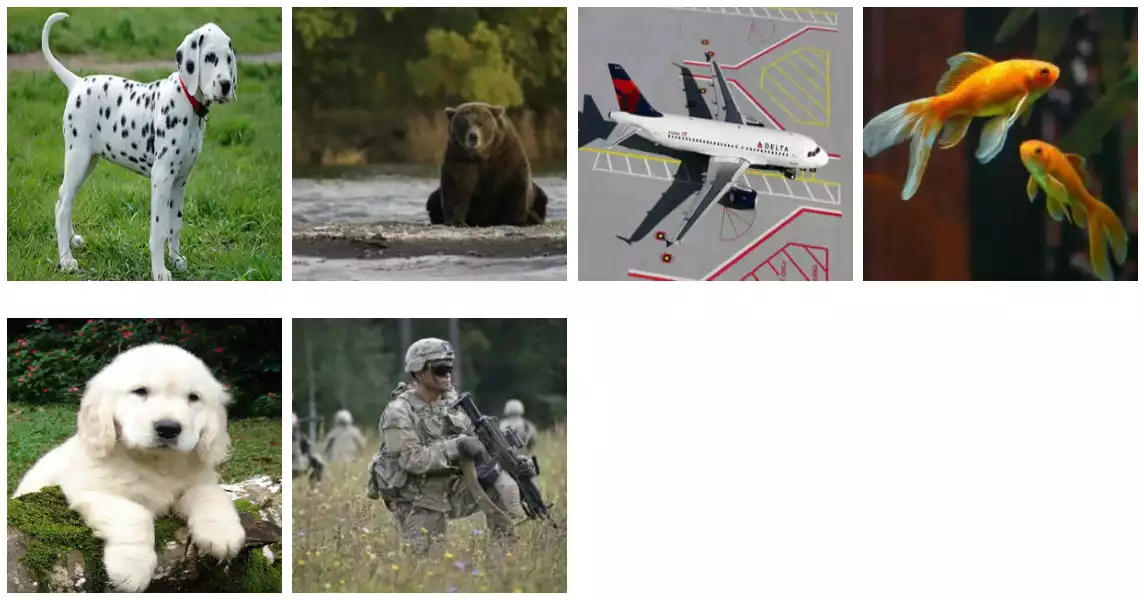
Let’s try and recreate these ideas using code. Consider the following input images – some extracted from the tf-keras-vis —, we will use them later and input for our methods.
INPUT_SHAPE = [299, 299, 3]

DATA_DIR = 'images/'
IMAGES = [
  'https://raw.githubusercontent.com/keisen/tf-keras-vis/master/examples/images/goldfish.webp',
  'https://raw.githubusercontent.com/keisen/tf-keras-vis/master/examples/images/bear.webp',
  'https://raw.githubusercontent.com/keisen/tf-keras-vis/master/examples/images/soldiers.webp',
  'https://3.bp.blogspot.com/-W__wiaHUjwI/Vt3Grd8df0I/AAAAAAAAA78/7xqUNj8ujtY/s400/image02.webp',
  'https://www.petcare.com.au/wp-content/uploads/2017/09/Dalmatian-2.webp',
  'http://www.aviationexplorer.com/Diecast_Airplanes_Aircraft/delta_Airbus_diecast_airplane.webp',
]
os.makedirs(os.path.join(DATA_DIR, 'test'), exist_ok=True)
for i in IMAGES:
    _, f = os.path.split(i)
    download_image(i, os.path.join(DATA_DIR, 'test', f))

images_set = tf.keras.preprocessing.image_dataset_from_directory(
  DATA_DIR, image_size=INPUT_SHAPE[:2], batch_size=32, shuffle=False)

images, labels = next(iter(images_set.take(1)))
In a real case, you would have your own trained network. However, considering all of these images belong to a class in the imagenet dataset, I’ll just go ahead and load the imagenet pre-trained Xception network from tensorflow. This will skip the training portion of the problem, which isn’t what we are focusing right now:
import tensorflow as tf
import tensorflow_addons as tfa

from tensorflow.keras import Sequential
from tensorflow.keras.layers import Lambda
from tensorflow.keras.applications.xception import (Xception,
                                                    preprocess_input,
                                                    decode_predictions)

# Download and load weights.
base_model = Xception(classifier_activation='linear',
                      weights='imagenet',
                      include_top=True)

model = Sequential([
    Lambda(preprocess_input),
    base_model
])

print_predictions(model, images, top=3)
Sample 0:
  dalmatian: 93.90%
  kuvasz: 0.14%
  Bernese_mountain_dog: 0.08%

Sample 1:
  brown_bear: 88.70%
  American_black_bear: 0.79%
  wombat: 0.52%

Sample 2:
  airliner: 93.20%
  wing: 1.11%
  warplane: 0.30%

Sample 3:
  goldfish: 73.91%
  tench: 0.54%
  gar: 0.19%

Sample 4:
  golden_retriever: 60.64%
  Great_Pyrenees: 8.80%
  kuvasz: 2.00%

Sample 5:
  assault_rifle: 65.17%
  bulletproof_vest: 11.51%
  rifle: 10.45%
So, as you can see, all samples have their classes correctly identified by the model with a large margin, compared with the second and third choices. Now we define a few utilitary functions to help us to run our algorithms:
UNIT_NAMES = [
  'dumbbell',
  'cup',
  'dalmatian',
  'bell_pepper',
  'lemon',
  'Siberian_husky',
  'computer_keyboard',
  'kit_fox',
]

LR = 10.
L2 = .1
TV = .1
STEPS = 200


def index_from(label):
    return int(next((k for k, v in imagenet_utils.CLASS_INDEX.items() if v[1] == label)))
And finally define our “vanilla” optimization process, using tensorflow’s GradientTape class:
def activation_gain(x, unit):
    y = model(x)
    return tf.reduce_mean(y[:, unit])

def l2_regularization(x):
    return tf.reduce_sum(tf.square(x), axis=(1, 2, 3), keepdims=True)

def total_var_regularization(x):
    return (tf.reduce_sum(tf.image.total_variation(x)
            / tf.cast(tf.reduce_prod(x.shape[1:-1]), tf.float32)))

@tf.function
def gradient_ascent_step(inputs, unit):
    with tf.GradientTape() as tape:
        tape.watch(inputs)

        loss = (activation_gain(inputs, unit)
                - L2 * l2_regularization(inputs)
                - TV * total_var_regularization(inputs))

    grads = tape.gradient(loss, inputs)
    grads = tf.math.l2_normalize(grads)
    inputs += LR * grads
    return loss, inputs

def visualize(unit):
    i = tf.random.uniform((1, *INPUT_SHAPE))
    i = (i - 0.5) * 0.25

    for step in range(STEPS):
        loss, i = gradient_ascent_step(i, unit)
        if step < STEPS - 1:
            i = tf.clip_by_value(i, -1, 1)

    return i
We can check if this process truly found maximizing images:
indices = [index_from(u) for u in UNIT_NAMES]

o = tf.concat([visualize(u) for u in indices], axis=0)
print_predictions(model, o, top=2)
Sample 0:
  dumbbell: 100.00%
  barbell: 0.00%

Sample 1:
  cup: 100.00%
  coffee_mug: 0.00%

Sample 2:
  dalmatian: 100.00%
  English_setter: 0.00%

Sample 3:
  bell_pepper: 100.00%
  cucumber: 0.00%

Sample 4:
  lemon: 100.00%
  orange: 0.00%

Sample 5:
  Siberian_husky: 100.00%
  Eskimo_dog: 0.00%

Sample 6:
  computer_keyboard: 100.00%
  mouse: 0.00%

Sample 7:
  kit_fox: 100.00%
  red_fox: 0.00%
plt.figure(figsize=(16, 9))
plot(as_image_vector(o), UNIT_NAMES, rows=2)
plt.tight_layout();
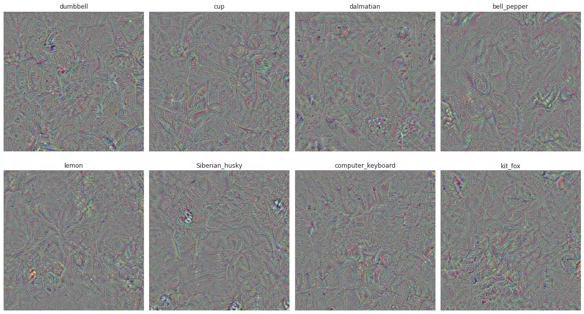
UNIT_NAMES.
I think I can see dumbells in the first image and dots in the dalmatian image, but I’m not sure if this is just my brain trying to look for evidence of correctness. Overall, I’d say it’s pretty hard to see the shapes in here and it doesn’t look like the results found in the paper (next image).
Differently from the original paper, I added a second regularization term
total variation, in order to decrease the amount of concentrated color regions in the generated images.
Lastly, I redefined visualize and added an “augmentation step” in each iteration,
where the optimizing image would be randomly rotated by 5% and translated by 3 pixels (at most).
This prevents the optimization procedure of focusting on single pixels and usually generate better images.
def visualize(unit):
    i = tf.random.uniform((1, *INPUT_SHAPE))
    i = (i - 0.5) * 0.25

    for step in range(STEPS):
        i = tfa.image.rotate(i, np.random.randn() * 0.05)
        i = tf.roll(i, (np.random.randn(2) * 15).astype(int), (1, 2))

        loss, i = gradient_ascent_step(i, unit)
        if step < STEPS - 1:
            i = tf.clip_by_value(i, -1, 1)

    return loss, i
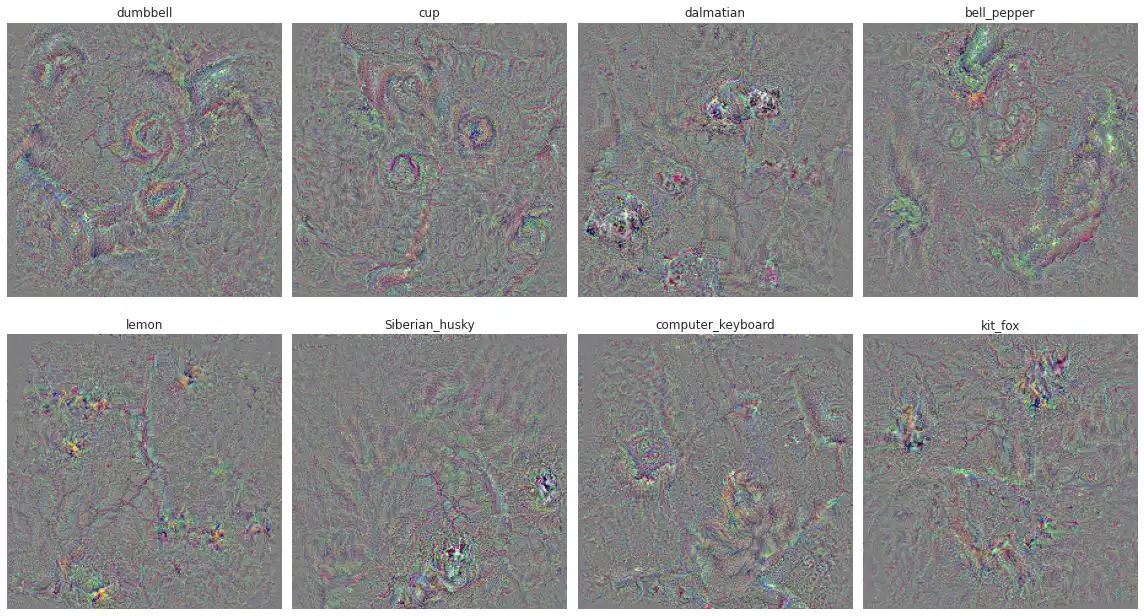
UNIT_NAMES using augmentation (rotation and translation).
It looks a lot better, I’d say. We see circles in dumbell, clear dark spots in dalmatian green in the bell pepper and lemon and squares in computer keyboard.
Contributions for The Classification of a Given Image
Another interesting idea in Deep Inside Convolutional Networks is the extraction of saliency maps using gradients. It works like this: let’s say $I$ is a real input image, $f$ a trained convolutional model and $S_c$ the activation value for the image true class $c$.
y = model(images)
y = tf.nn.softmax(y)
p = tf.argmax(y, axis=-1)
pr = tf.reduce_max(y, axis=-1)
Once again, assuming that this model can be sufficiently approximated by a first-order Taylor expansion. That is,
\[\begin{eqnarray} S_c &=& f(I)_c \\ &\approx& \sum_i \sum_j \frac{\partial S_c(I)}{\partial I_{i,j}} I_{i,j} \end{eqnarray}\]$\frac{\partial S_c(I)}{\partial I}$ is an approximation of how each pixel in the input image $I$ contributes to the output of the model. Three possibilities here:
- If the contribution is close to $0$, then that pixel contributes little and any variations.
- If the number is strongly positive, then high values for that pixel contribute to its correct classification.
- If the number is strongly negative, then low values for that pixel contribute to its correct classification.
So we first must find $\frac{\partial S_c(I)}{\partial I}$. That’s pretty simple. I just copied the important part from what we did above (and changed the activation_gain function a bit so it could process multiple samples at the same time):
def activation_gain(inputs, units):
    y = model(inputs)
    return tf.gather(y, units, axis=1, batch_dims=1)

@tf.function
def gradients(inputs, units):
    with tf.GradientTape() as tape:
        tape.watch(inputs)
        loss = activation_gain(inputs, units)

    grads = tape.gradient(loss, inputs)

    return loss, grads
Finally, we observe which pixels are most important when classifying the image label by considering their absolute value (added across its RGB channels):
_, g = gradients(images, p)

s = tf.reduce_sum(tf.abs(g), axis=-1)
s /= tf.reduce_max(s, axis=(1, 2), keepdims=True)

plot_images_and_salency_maps(as_image_vector(images), s.numpy(), y.numpy())
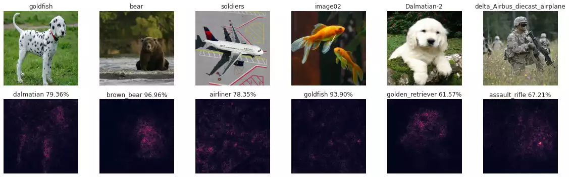
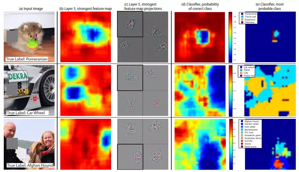
So the network clearly points out for the right regions in the dalmatian, bear and the golden retriever. The other ones seem a little blurred.
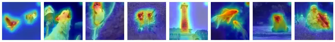
Smooth Gradients
An improvement for this strategy is described in SmoothGrad: removing noise by adding noise. In the article, the authors comment that gradients may vary sharply at small scales due to meaningless variations in small portions of the input space, generating a misrepresentation of pixels’ importances. They propose to overcome this issue by generating $N$ repetitions of the input image $I$ and add some gaussian noise to each one of them. The gradients are then computed with respect to each repetition, and the maps found are averaged into a single representation.
With that, enough fluctuation will be generated in the input image. Hence local artificial variations will not ocurr in many of the gradients found and will be phased out from the final averaging map.
Code is pretty straight forward. We use the arguments which produced good results, as described in the article (50 repetitions, 20% noise). Notice that we have divided the input noise by $2.0$ (sample inner variation $x_{\text{max}} - x_{\text{min}}$), in order to match the definition given in the paper.
@tf.function
def smooth_gradients(inputs, units, num_samples=50, noise=.2):
  x = tf.repeat(inputs, num_samples, axis=0)
  x += tf.random.normal(x.shape, mean=0, stddev=noise / 2)

  y = tf.repeat(units, num_samples)
  loss, grads = gradients(x, y)

  grads = tf.reshape(grads, (-1, num_samples, *grads.shape[1:]))

  return loss, tf.reduce_mean(grads, axis=1)
_, g = smooth_gradients(images, p, num_samples=20)

s = tf.reduce_sum(tf.abs(g), axis=-1)
s /= tf.reduce_max(s, axis=(1, 2), keepdims=True)
plot_images_and_salency_maps(as_image_vector(images), s.numpy(), y.numpy())

Much better, isn’t it?
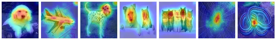
Full Gradients
Another interesting idea can be found in the article Full-gradient representation for neural network visualization. This approach’s main idea is to combine the saliency information previously found with the individual contributions of each bias factor in the network, forming a “full gradient map”:
\[f(x) = ψ(∇_xf(x)\odot x) +∑_{l\in L}∑_{c\in c_l} ψ(f^b(x)_c)\]We can extract the bias tensor from most layers in a TensorFlow model by accessing tehir layer.bias attribute.
The Batch-Norm layer, however, has what we call an implict bias.
Let the Batch-Norm (BN) of a input signal $x$ be $\text{bn}(x) = \frac{x - \mu}{\sigma}w + b$, then its rectified bias is $b^r = -\frac{\mu}{\sigma}w + b$.
All of this is expressed in the following python code:
def activation_gain(y, units):
    return tf.gather(y, units, axis=1, batch_dims=1)

def extract_bias(layer):
  if isinstance(layer, tf.keras.layers.BatchNormalization):
    return (
        -layer.moving_mean * layer.gamma
        / tf.sqrt(layer.moving_variance + 1e-07)
        + layer.beta)

  if hasattr(layer, 'bias') and layer.bias is not None:
    return layer.bias

def psi(x):
  x = tf.abs(x)
  x = standardize(x)

  return x

layers = [(l, extract_bias(l)) for ix, l in enumerate(nn.layers[1:-1])]
layers = [(l, b) for l, b in layers if b is not None]

intermediates = [l.output for l, _ in layers]
biases = [b for _, b in layers]

print(len(biases), 'layers with bias were found.')

nn_s = tf.keras.Model(nn.inputs, [nn.output, *intermediates], name='spacial_model')
@tf.function
def fullgrads(inputs, units):
  with tf.GradientTape() as tape:
    tape.watch(inputs)
    y, *ia = nn_s(inputs, training=False)
    loss = activation_gain(y, units)

  dydx, *dydas = tape.gradient(loss, [inputs, *ia])

  maps = tf.reduce_sum(psi(dydx * inputs), axis=-1)

  Gb = [ig * tf.reshape(b, (1, 1, 1, -1)) for ig, b in zip(dydas, biases)]
  for b in Gb:
      b = psi(b)
      maps += tf.reduce_sum(tf.image.resize(b, config.data.image_size), axis=-1)

  return loss, dydx, maps
r = zip(*[fullgrads(x[ix:ix+1], preds[ix:ix+1]) for ix in range(len(images))])
_, g, maps = (tf.concat(e, axis=0) for e in r)

maps = normalize(maps)

s = normalize(tf.reduce_sum(tf.abs(g), axis=-1))

def plot_heatmaps(images, maps, rows=1, cols=None, i0=0, full=True):
    if full: plt.figure(figsize=(16, 4 * rows))
    for ix, (i, m) in enumerate(zip(images, maps)):
        plt.subplot(rows, cols or len(images), i0+ix+1)
        plot_heatmap(i, m)
    if full: plt.tight_layout()

def plot_heatmap(i, m):
    plt.imshow(i)
    plt.imshow(m, cmap='jet', alpha=0.5)
    plt.axis('off')

plot_heatmaps(to_image(images), maps)
Final Considerations
AI explaining is a very long subject, containing many different strategies. In this post, I illustrated a illustrates a few examples of it and briefly explains how classification gradient can be used to explain predictions in Computer Vision.
This is pretty much an open research field, with many methods coming to light in the past years. Some filter the back-propagated signal, in order to only capture what positively affects the output (Guided backpropagation). Others will focus on general localization instead of fine-gain details (CAM), resulting in maps that better separates classes coexisting in a single sample. I’ll talk a little bit more about these in the next post.
References
- Simonyan, Karen, Andrea Vedaldi, and Andrew Zisserman. “Deep inside convolutional networks: Visualising image classification models and saliency maps.” arXiv preprint arXiv:1312.6034 (2013). 1312.6034
- Smilkov, Daniel, Nikhil Thorat, Been Kim, Fernanda Viégas, and Martin Wattenberg. “Smoothgrad: removing noise by adding noise.” arXiv preprint arXiv:1706.03825 (2017). 1706.03825
- Srinivas, Suraj, and François Fleuret. “Full-gradient representation for neural network visualization.” arXiv preprint arXiv:1905.00780 (2019). 1905.00780