Class Activation Mapping

In my last post, I talked about AI explaining in the computer vision area, and how to use the gradient information to explain predictions for classification networks. In short, if we consider our answer to be $a(x) = \max f(x)$, for whatever differentiable network $f$ and input image $x$, we should be able to compute $\nabla a$. I.e., the gradient with respect to the input $x$, composing a map of linear contributions for each RGB value of each pixel in the image. Furthermore, we can obtain smooth gradients by repeating this process $N$ times, adding a little noise each time. 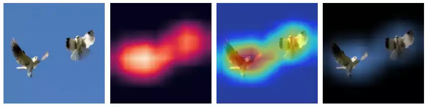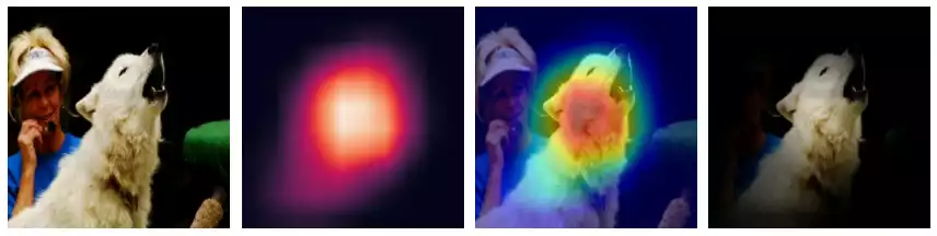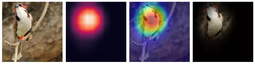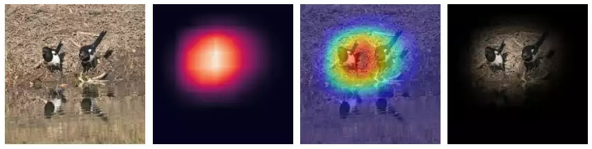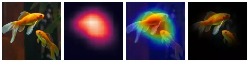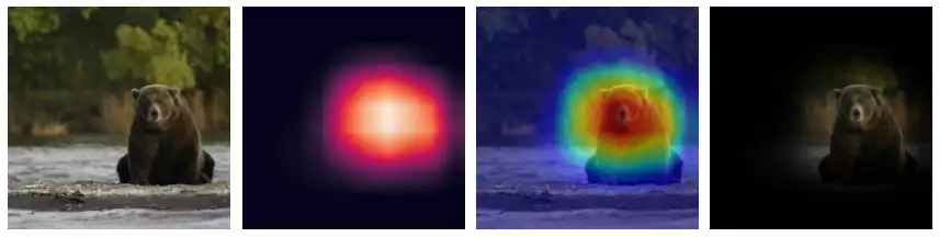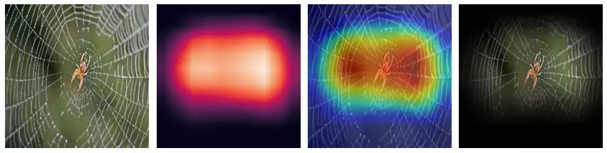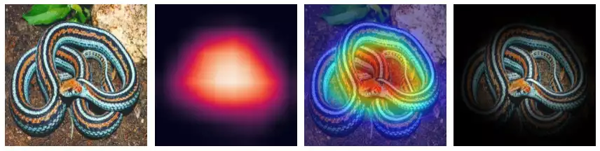The images below describe the application of VanillaGrad and SmoothGrad over multiple images.

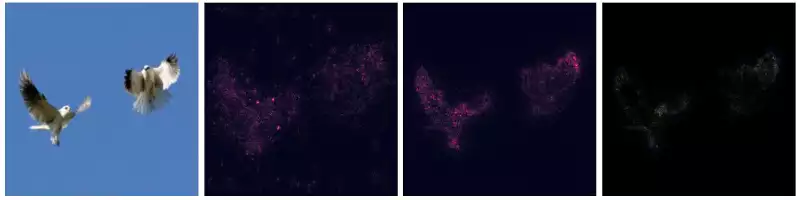
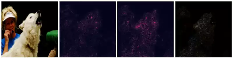
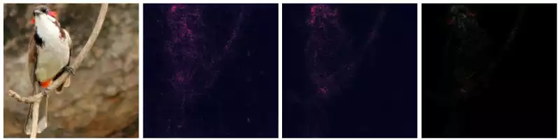
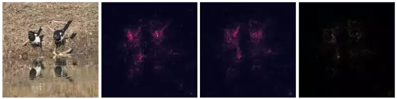
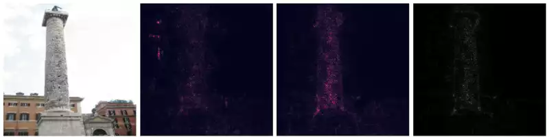
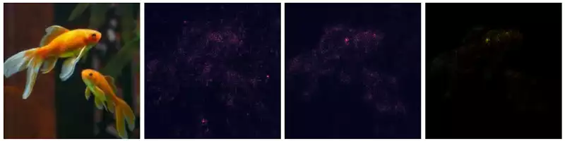
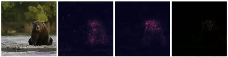
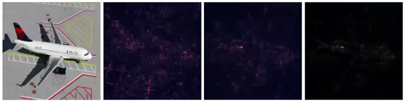
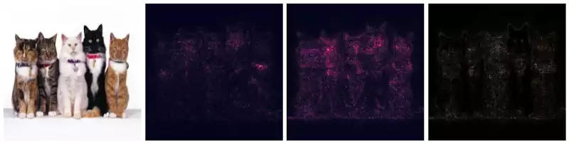
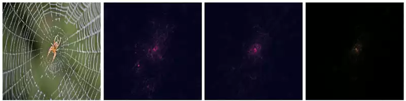
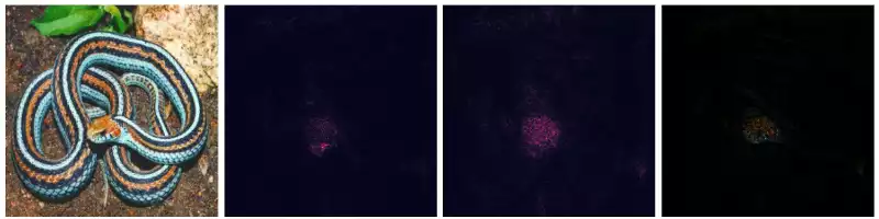
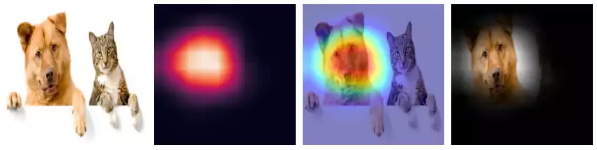
This works pretty well for images containing a single entity of the classifying set (e.g. the birds, the fish). However, things become a little messy then the image contains multiple elements. For example:

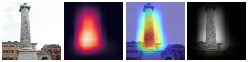
In the image of the dog, classified as 84.7% white wolf, 3.2% kuvasz and 3.0% timber wolf, the gradients highlight the human being as well.
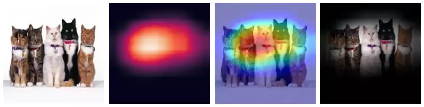
In the obelisk image (classified as obelisk), large portions of the buildings are highlighted by both Vanilla and SmoothGrad methods.
The image containing multiple cat species was classified as 43.8% tabby, 27.2% Egyptian cat, 6.0% tiger cat and 2.7% Persian cat. However, the gradients with respect to tabby extend to all cats, not only the tabby species.

So it’s clear that gradient-based methods are not class-discriminative, as not only sections of the object represented by the output unit are highlighted, but also sections of related objects and other classes belonging to the set.

Class Activation Mapping (CAM)

Going in a different direction, a method that focus on class separation was proposed for understanding convolutional networks, called CAM [1].

CAM only apply to convolutional networks with a single densely connected softmax layer at its end, without bias value attached. The TF code for such network looks something like this:

import tensorflow as tf
from tensorflow.keras import Input, Model, layers

C = 1584

backbone = tf.keras.applications.EfficientNetB7(include_top=False)

x = Input((600, 600, 3), name='images')
y = backbone(x)
y = layers.Dense(C, use_bias=False, name='predictions')(y)

network = Model(x, y)
network.compile(..., loss=tf.losses.SparseCategoricalCrossentropy(from_logits=True))

Let $f$ by a network as proposed above, $x$ be an input signal (image), $A_{i,j}^k$ the spatial activation signal from the last convolutional layer in $f$ and $S_u$ the activation strength of any classifying unit $u$ of the softmax layer:

\[\begin{align} S_u(x) &= \sum_k w_{u,k} \frac{1}{N} \sum_{i,j} A_{i,j}^k \\ &= \frac{1}{N}\sum_{i,j} \sum_k w_{u,k} A_{i,j}^k \end{align}\]

Where the importance of each spatial unit $A_{i,j}^k$ is $w_{u,k}$. The definition of importance map follows directly from it:

\[M(f, x, u) = \text{upsample}(\sum_k w_{u,k} A_{i,j}^k)\]

The upsample function refers to the resizing procedure of the map to the input image’s original sizes. Because networks tend to reduce their intermediate signal considerably, with respect to the spatial components (EfficientNetB4, for instance, reduces images $300\times 300\times 3$ to $10\times 10\times 1792$), a considerable amount of precision is lost in this step. Hence, this method can only find coarse regions of interest.

From the equations, we can see this signal does not have an upper bound, and might present arbitrarily large numbers. We can build an attention map by normalizing it across the spatial components. This normalization also removes the constant $N$ from the eq.

Grad-CAM

A second article [2], written by researchers at George Institute of Technology, addresses the architecture limitations set by CAM. In it, they combine gradient-based saliency and CAM to replace the $w_{u,k}$ importance factor described above by the differential of the activating unit with respect to the activating signal.

To derive this, consider the equation for CAM’s network’s output once again:

\[\begin{align} S_u(x) &= \sum_k w_{u,k} P(A_{i,j})^k \\ P(A)^k &= \frac{1}{N} \sum_{i,j} A_{i,j}^k \end{align}\]

Term $w_{u,k}$ is the contribution of filter $k$ to the classification of label $u$. In a non linear case, we can approximate it from the differential of the activation unit $u$ with respect to the activation map $A_{i,j}^k$:

\[\begin{align} \frac{\partial S_u(x)}{\partial A_{i,j}^k} &= \frac{\partial S_u(x)}{\partial P^k} \frac{\partial P^k}{\partial A_{i,j}^k}\\ \iff \frac{\partial S_u(x)}{\partial P^k} &= \frac{\frac{\partial S_u(x)}{\partial A_{i,j}^k}}{\frac{\partial P^k}{\partial A_{i,j}^k}} \\ \end{align}\]

But $\frac{\partial P^k}{\partial A_{i,j}^k} = \frac{1}{N}$ and $\frac{\partial S_u(x)}{\partial P^k} = w_{u,k}$, hence:

\[\begin{align} w_{u,k} &= N \frac{\partial S_u(x)}{\partial A_{i,j}^k} \\ \implies N w_{u,k} &= N \sum_{i,j} \frac{\partial S_u(x)}{\partial A_{i,j}^k}\\ \implies w_{u,k} &= \sum_{i,j} \frac{\partial S_u(x)}{\partial A_{i,j}^k} \end{align}\]

Lastly, the authors only consider the pixels with positive influence over the classification unit $u$, ignoring channels with negative contribution. The entire eq. can be expressed as:

\[M(f, x, u)_{i,j} = \text{upsample}(\sum_k \text{relu}(\sum_{l,m}\frac{\partial S_u}{\partial A_{l,m}^k}) A_{i,j}^k)\]

Because the contributions of each kernel in the last convolution are estimated with the gradient information, we can generalize this attention method to any kind of network. The paper exemplifies it with a network that combine Conv2D with LSTM layers to generate natural textual descriptors from images.

TensorFlow’s implementation of Grad-CAM is pretty simple. We start by defining the network: as a multi-output network, which feeds on images and outputs the classification logits and the positional signal from the last spatial layer (our signal $A$). Finally, we feed-forward the images through it.

LAST_SPATIAL_LAYER = 'block14_sepconv2_act'

nn = tf.keras.applications.Xception()

ss = tf.keras.Model(
    inputs=nn.inputs,
    outputs=[nn.output, nn.get_layer(LAST_SPATIAL_LAYER).output],
    name='spatial')

images = read_images(...)
features = images / 127.5 - 1  # Normalize input-signal to (-1, 1), expected by Xception.

logits = nn(features, training=False)
preds = tf.argmax(logits, axis=1)
probs = tf.nn.softmax(logits)

And finally, we define our gradcam function:

def activation_gain(y, units):
    return tf.gather(y, units, axis=1, batch_dims=1)

@tf.function
def gradcam(inputs, units):
    with tf.GradientTape(watch_accessed_variables=False) as tape:
        tape.watch(inputs)
        y, z = ss(inputs, training=False)
        loss = activation_gain(y, units)

    grads = tape.gradient(loss, z)
    weights = tf.reduce_mean(grads, axis=(1, 2), keepdims=True)
    maps = tf.reduce_mean(z*weights, axis=-1, keepdims=True)

    # We are not concerned with pixels that negatively contribute
    # to its classification, only pixels that belong to that class.
    maps = tf.nn.relu(maps)
    maps = normalize(maps)
    maps = tf.image.resize(maps, (600, 600))

    return loss, maps[..., 0] # (H, W, 1) --squeezed--> (H, W)

def normalize(x):
    x -= tf.reduce_min(x, axis=(1, 2), keepdims=True)
    x /= tf.reduce_max(x, axis=(1, 2), keepdims=True) + 1e-07
    return x

Notice we need the arguments axis=1, batch_dims=1 in tf.gather because the tf.argmax operation returned a tensor with a different number of ranks from y. A valid alternative is to remove these args and reshape preds as a column vector.

Lastly, we only need to call gradcam using our input images and units of interest:

loss, maps = gradcam(features, preds)

def plot_heatmaps(images, maps, rows=1, cols=None, i0=0, full=True):
    if full: plt.figure(figsize=(16, 4 * rows))
    for ix, (i, m) in enumerate(zip(images, maps)):
        plt.subplot(rows, cols or len(images), i0+ix+1)
        plot_heatmap(i, m)
    if full: plt.tight_layout()

def plot_heatmap(i, m):
    plt.imshow(i)
    plt.imshow(m, cmap='jet', alpha=0.5)
    plt.axis('off')


plot_heatmaps(images, maps)

That’s it! Hopefully you can re-use this in your own networks! (-:

I have written a AI explaining library that contains many of the visualization techniques (including Grad-CAM) out of the box. You can check it out here: lucasdavid.github.io/keras-explainable/

References

B. Zhou, A. Khosla, A. Lapedriza, A. Oliva, and A. Torralba, “Learning deep features for discriminative localization,” in IEEE conference on Computer Vision and Pattern Recognition (CVPR), 2016, pp. 2921–2929.
R. R. Selvaraju, M. Cogswell, A. Das, R. Vedantam, D. Parikh, and D. Batra, “Grad-CAM: Visual explanations from deep networks via gradient-based localization,” in IEEE conference on Computer Vision and Pattern Recognition (CVPR), 2017, pp. 618–626.