Activation, Cross-Entropy and Logits

Activation and loss functions are paramount components employed in the training of Machine Learning networks. In the vein of classification problems, studies have focused on developing and analyzing functions capable of estimating posterior probability variables (class and label probabilities) with some degree of numerical stability. In this post, we present the intuition behind these functions, as well as their interesting properties and limitations. Finally, we also describe efficient implementations using popular numerical libraries such as TensorFlow.

show setup code

import numpy as np
import pandas as pd

import tensorflow as tf
from tensorflow.keras import layers

import matplotlib.pyplot as plt
import seaborn as sns

sns.set(style='whitegrid')

class Config:
  batch_size = 256
  shape = (32, 32, 3)

Activation Functions

Classification networks will often times employ the softmax or sigmoid activation functions in their last layer:

from tensorflow.keras.layers import Dense

features = np.asarray(
  [[0.1,  0.2, 5.1, ...],
   [2.6, -0.4, 1.1, ...],
   ...])
labels = ['label_01', 'label_02', 'label_03', ...]

nn = tf.keras.Sequential([
  Dense(1024, activation='swish', name='fc1'),
  Dense(1024, activation='swish', name='fc2'),
  Dense(len(np.unique(labels)), activation='softmax', name='predictions'),
])

These functions are useful to limit the output of the model to conform with the expected predicted variable, which likely model a posterior probability distribution or a multi-variate probability distribution signal.

Sigmoid

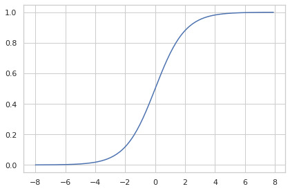
The sigmoid function has a historical importance to Machine Learning, being commonly employed in the classic connectionist approach of Artificial Intelligence (Multi-layer Perceptron Networks) for its interesting properties [1]. Firstly, it is bounded to the real interval $[0, 1]$, and differentiable on each and every point of its domain. It is monotonically increasing, which means it does not affect the rank between the input logits ($\arg\max_i S(x) = \arg\max_i x$) [1]. It’s derivative is a bell function, with the highest value in 0. It is convex in $[-\infty, 0]$ and concave $[0, \infty]$ [1], so it saturates when outputting close to its extremities.

Let $l = x\cdot w + b$ be the result of the last dense layer in the network (the inner product between an input feature vector and the weights vector of the layer, added to the bias factor), commonly referred to as the logit vector in the Machine Learning literature. The sigmoid function is defined as:

And it looks like this:

x = tf.reshape(tf.range(-8, 8, delta=.1), (-1, 1))
y = tf.nn.sigmoid(x)

show code

sns.lineplot(x=x.numpy().ravel(), y=y.numpy().ravel())
plt.tight_layout();

In Mathematics, the logit (logistic unit) function is the inverse of the sigmoid function [2]:

Jacobian

The sigmoid function does not associate different input numbers, so it does not have cross-derivatives with respect to the inputs, and thus, $\text{diag}(\nabla S) = \mathbf{J} S$.

And,

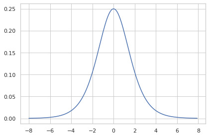
Softmax

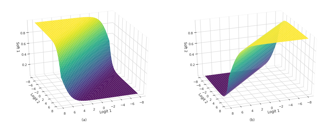
The softmax function is defined as [3]:

This function has some interesting properties as well. Firstly, it is monotonically increasing. Hence, $\arg \max_i \text{softmax}(x) = \arg \max_i x$. Secondly, it’s strictly positive, and it will always output a vector that adds up to 100%, regardless of the values in $l$. Lastly, it is quickly saturated, so small changes in the input distribution (e.g. weights) cause a large shift in the output distribution (predictions). In other words, it can be quickly trained.

z = tf.stack(tf.meshgrid(x, x), axis=-1)
y = tf.nn.softmax(z)

show code

def show_sm_surface(ax, a, b, y, sm=0, title=None):
  ax.plot_surface(a, b, y[..., sm], cmap=plt.cm.viridis, linewidth=0.1)
  ax.view_init(30, 70)

  ax.set_xlabel("Logit 1")
  ax.set_ylabel("Logit 2")
  ax.set_zlabel(f"Soft {sm+1}")
  ax.xaxis.pane.fill = False
  ax.yaxis.pane.fill = False
  ax.zaxis.pane.fill = False

  if title: plt.title(title, y=-0.05)

fig = plt.figure(figsize=(16, 6))
show_sm_surface(fig.add_subplot(121, projection = '3d'), a, b, y, sm=0, title='(a)')
show_sm_surface(fig.add_subplot(122, projection = '3d'), a, b, y, sm=1, title='(b)')

plt.tight_layout();

Jacobian

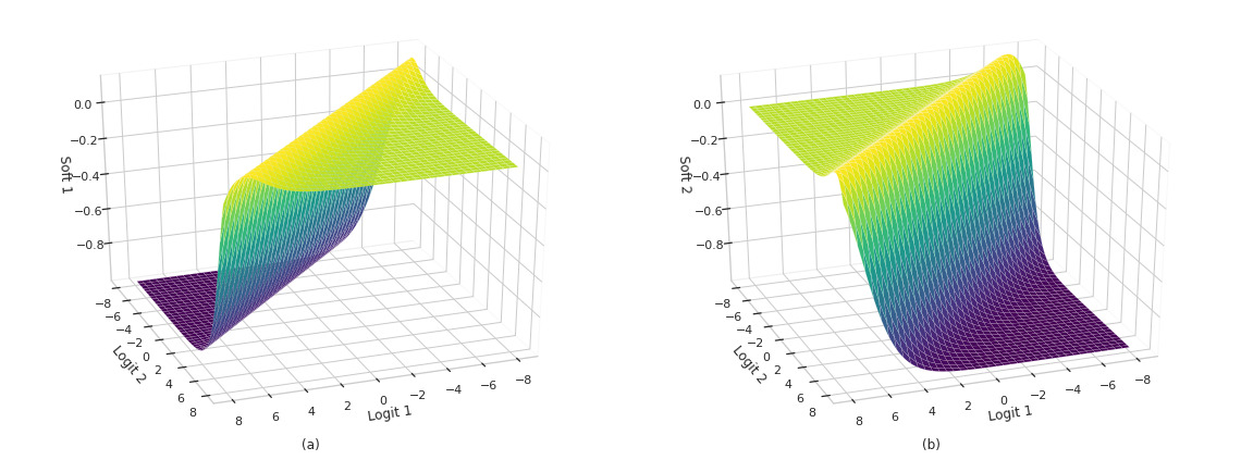
While the softmax function preserves the shape of the input vector, each output element is formed by the combination of all input elements. This clearly hints that the Jacobian of the softmax function is a full matrix.

The the Jacobian of the softmax function $\mathbf{J} \text{softmax}$ can be computed in two steps. Firstly, for the elements in the main diagonal:

Using the quotient rule:

For the elements outside of the main diagonal:

Then,

Where $\text{sm}_i = \text{softmax}_i(x)$.

z = tf.stack(tf.meshgrid(x, x), axis=-1)
y = tf.nn.softmax(z)
i = tf.eye(2)

y = y[..., tf.newaxis]

y_grad = y * (i-y)
y_grad = tf.reduce_sum(y_grad, axis=-1)

show code

fig = plt.figure(figsize=(16, 6))
show_sm_surface(fig.add_subplot(121, projection = '3d'), a, b, y_grad, sm=0, title='(a)')
show_sm_surface(fig.add_subplot(122, projection = '3d'), a, b, y_grad, sm=1, title='(b)')

plt.tight_layout();

Comparison with Normalized Logits

In a first thought, a simple normalization could also be used as activation function in classification models, while holding the first two properties described above:

def normalized_logits(x, axis=-1):
  x -= tf.reduce_min(x, axis=axis, keepdims=True) - 1e-7
  x /= tf.reduce_sum(x, axis=axis, keepdims=True) + 1e-7

  return x

It wouldn’t be as fast to train or as stable as softmax, though:

show code

import tensorflow as tf
from tensorflow.keras import layers

class Config:
  batch_size = 256
  shape = (32, 32, 3)

# Dataset
(x_train, y_train), (x_test, y_test) = tf.keras.datasets.cifar10.load_data()

# Model
preprocessing = tf.keras.Sequential([
  tf.keras.layers.RandomFlip("horizontal"),
  tf.keras.layers.RandomRotation(0.1),
  tf.keras.layers.experimental.preprocessing.Rescaling(1./127.5, offset=-1),
])

def make_model(
    input_shape,
    num_classes,
    top_activation='softmax'
):
  """Build a convolutional neural network using skip-connections and Separable Conv2D Layers.

  Ref: https://keras.io/examples/vision/image_classification_from_scratch/

  """
  inputs = tf.keras.Input(shape=input_shape)
  x = preprocessing(inputs)

  # Entry block
  x = layers.Conv2D(32, 3, strides=2, padding="same")(x)
  x = layers.BatchNormalization()(x)
  x = layers.Activation("relu")(x)

  x = layers.Conv2D(64, 3, padding="same")(x)
  x = layers.BatchNormalization()(x)
  x = layers.Activation("relu")(x)

  previous_block_activation = x  # Set aside residual

  for size in [128, 256]:
    x = layers.Activation("relu")(x)
    x = layers.SeparableConv2D(size, 3, padding="same")(x)
    x = layers.BatchNormalization()(x)

    x = layers.Activation("relu")(x)
    x = layers.SeparableConv2D(size, 3, padding="same")(x)
    x = layers.BatchNormalization()(x)

    x = layers.MaxPooling2D(3, strides=2, padding="same")(x)

    # Project residual
    residual = layers.Conv2D(size, 1, strides=2, padding="same")(
        previous_block_activation
    )
    x = layers.add([x, residual])  # Add back residual
    previous_block_activation = x  # Set aside next residual

  x = layers.SeparableConv2D(1024, 3, padding="same")(x)
  x = layers.BatchNormalization()(x)
  x = layers.Activation("relu")(x)

  x = layers.GlobalAveragePooling2D(name='avg_pool')(x)
  x = layers.Dropout(0.5, name='head/drop')(x)
  outputs = layers.Dense(num_classes, activation=top_activation, name='head/predictions')(x)
  return tf.keras.Model(inputs, outputs)

def train(
  top_activation,
  optimizer,
  loss,
  epochs = 18,
):
  model = make_model(input_shape=Config.shape, num_classes=len(np.unique(y_train)), top_activation=top_activation)
  model.compile(optimizer=optimizer, loss=loss, metrics=["accuracy", 'sparse_top_k_categorical_accuracy'])
  model.fit(
    x_train, y_train,
    epochs=epochs,
    validation_data=(x_test, y_test)
  );

  return pd.DataFrame(model.history.history)

history_softmax = train(
  top_activation=tf.nn.softmax,
  optimizer=tf.optimizers.SGD(),
  loss=tf.losses.SparseCategoricalCrossentropy()
)

history_normalized_logits = train(
  top_activation=normalized_logits,
  optimizer=tf.optimizers.SGD(),
  loss=tf.losses.SparseCategoricalCrossentropy()
)

show code

import matplotlib.pyplot as plt
import seaborn as sns

sns.set()


def plot_accuracy_lines(*histories):

  plt.figure(figsize=(16, 4))


  for i, (h, name) in enumerate(histories):
    plt.subplot(1, len(histories), i + 1)
    plt.title(name)
    sns.lineplot(data=h.reset_index().rename(columns={
                        'index': 'epoch',
                        'accuracy': 'top 1 score training',
                        'sparse_categorical_accuracy': 'top 1 score training',
                        'val_accuracy': 'top 1 score validation',
                        'val_sparse_categorical_accuracy': 'top 1 score validation',
                        'sparse_top_k_categorical_accuracy': 'top 5 score training',
                        'val_sparse_top_k_categorical_accuracy': 'top 5 score validation',
                      }).melt(
                        ['epoch'],
                        ['top 1 score training', 'top 1 score validation', 'top 5 score training', 'top 5 score validation'],
                        'metric'),
      x='epoch',
      y='value',
      hue='metric'
    );

plot_accuracy_lines(
  (history_softmax, 'Softmax'),
  (history_normalized_logits, 'Normalized Logits'),
)

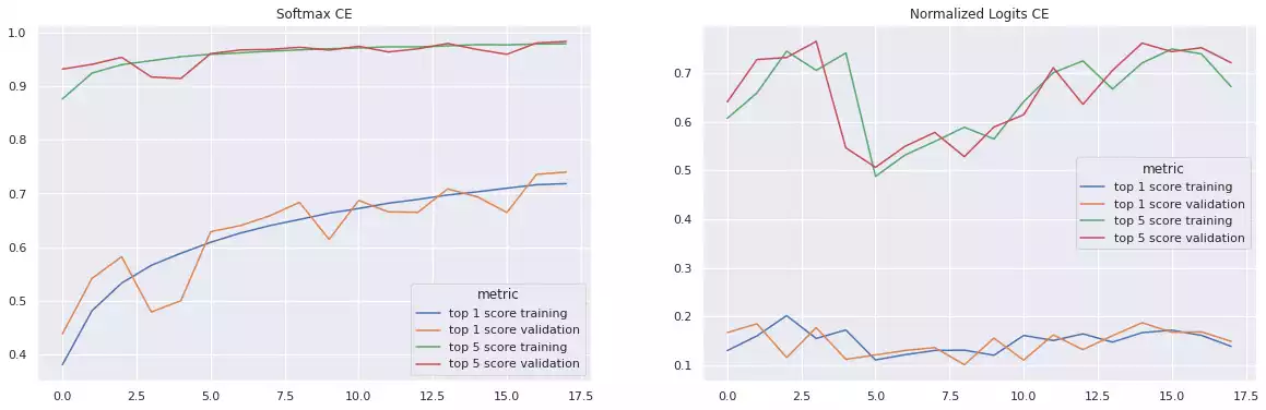
The log function inside the Cross-entropy function counteracts the exponential inside the softmax function (see the Categorical Cross-entropy with Logits Section below), implying that the gradient of the loss function with respect to the logits are somewhat linear in $l_i$ [4], allowing for the model to update its weights at a reasonable pace. By replacing the activation function by a linear normalization (while using Categorical Cross-entropy), the weights are now being updated at a logarithmic rate. Finally, changing the loss function to something else (like Mean Squared Error) fixes the aforementioned issue, but creates many other problems, such as: (a) the error function is no longer bonded; (b) it is slower to train, as small changes in weights no longer produce large changes in the output; and (c) saturation no longer occurs after a considerate amount of epochs, introducing instability to the training procedure.

Stability Tricks

It’s worth remarking that the $e^x$ function can result in numerical under/overflow, if its inputs are very large numbers [5]. However, this can be easily remedied by remembering that this function is invariant to translations in its domain.

Let $C\in\mathbb{R}$ be a constant factor, then

So it’s quite common for computing tools to define the softmax function as $\text{softmax}(l - \max_i l)_i$, implying $l - \max(l) \le 0 \implies e^l_i \le 1$:

def softmax(x, axis=-1):
  x -= tf.reduce_max(x, axis=axis, keep_dims=True)
  x = tf.math.exp(x)

  return tf.math.divide_no_nan(
    x,
    tf.reduce_sum(x, axis=axis, keep_dims=True)
  )

# Or tf.nn.softmax

Underflow might still happen after shifting the input, if the logits greatly differ. This is highly unlikely, though, as all of the parameters are randomly drawn from the same random distribution and small changes are expected during training.

Losses

In this section, I list two very popular forms of the cross-entropy (CE) function, commonly employed in the optimization (or training) of Network Classifiers.

Categorical Cross-Entropy

The Categorical CE loss function is a famous loss function when optimizing estimators for multi-class classification problems [6]. It is defined as:

This function is also called negative log likelihood, and it is heavily based on the eq. of Information Entropy proposed by Shannon [7].

In TensorFlow’s notation [8], we can write it as:

def categorical_crossentropy(y, p):
  return -tf.reduce_sum(y * p, axis=-1)

# Or simply tf.losses.categorical_crossentropy

Quite simple. Notice this might not return a single real number, as the operation mean is applied over a single dimension (the last one). In fact, for the common case of a Multilayer Perceptron Network, y and p are matrices of shapes [batch, labels] and mean-reducing their pairwise multiplication will result in a vector of shape [batch]. However, when calling for the GradientTape#gradient with anything but a number, TensorFlow will internally summarize this same tensor into a single number by add-reducing all of its elements. Conversely, the gradient of each element in a tensor with respect to the inputs can be obtained from the methods GradientTape#jacobian and GradientTape#batch_jacobian.

The gradients of the trainable weights can be retrieved using a GradientTape. Parameters can then be updated using an Optimizer:

def train_step(model, x, y):
  with tf.GradientTape() as tape:
    p = network(x, training=True)

    loss = categorical_crossentropy(y, p)

  trainable_variables = network.trainable_variables
  gradients = tape.gradient(loss, trainable_variables)

  optimizer.apply_gradients(zip(gradients, trainable_variables))

While some shenanigans occur inside the optimizer (like keeping track of moving averages, normalizing vectors by dividing them by their $l^2$-norm), the optimizer will ultimately minimize the loss function by subtracting the gradients to the parameters themselves (docs on Optimizer), walking the in the direction of steepest descent of the optimization manifold.

Intuition

Categorical CE can be interpreted as a sum of the log probabilities conditioned to the association of the sample to the respective class being predicted. If $y_i = 0$ (i.e., the sample does not belong to the class $i$), then the output $p_i$ is ignored in the optimization process. Conversely, if the association exists, then $y_i = 1$, hence:

It’s important to keep in mind that this isn’t the same as saying that the logit $l_i$ will be ignored, as it also appears in the denominator of the softmax function in the terms $p_j \mid j \ne i$.

Without loss of generality, the log of a ratio is always negative:

Categorical CE is minimum when the probability factor $p_i = 1, \forall i \mid y_i = 1$, and grows as the classification probability decreases. Therefore, the Optimizer instance minimizes the loss function by increasing the classification probability $p_i$ of a sample associated with the class $y_i$.

Sparse Categorical CE

In the simplest case, a multi-class and single-label problem, $y$ is a one-hot encoded vector (in which all elements but one are zero), and thus can be more efficiently represented as a single positive integer, representing the associated class index. I.e., we assume y to be a vector of shape [batch] and p the common [batch, classes]. Therefore:

This form, commonly known as Sparse CE, can be written in the following way in TensorFlow:

def sparse_categorical_crossentropy(y, p, axis=-1):
  p = tf.gather(p, y, axis=axis, batch_dims=1)
  p = -tf.math.log(p)

  return p

# Or simply tf.losses.sparse_categorical_crossentropy

Notice we no longer add all of the elements of the probability vector $p$ (as all of them are multiplied by 0 and would not change the loss value). This is not only more efficient, but also induces more numerical stability by generating a smaller computation graph.

Categorical CE from Logits

Finally, I think we are ready to go over this! It’s quite simple, actually. We need only to expand the Categorical CE and softmax equations above.

Let $x\in X$ be a feature vector representing sample in the set $X$, $l$ be the logits vector and $p = \text{softmax}(l)$. Furthermore, let $y$ be the ground-truth class vector associated with $x$. Then,

Applying $\log (q/t) = \log q - \log t$,

Hence, we can merge the softmax and Categorical CE functions into a single optimization equation:

def softmax_cross_entropy_with_logits(y, l, axis=-1):
  return -tf.reduce_sum(
    y * (l + tf.math.log(tf.reduce_sum(tf.math.exp(l), axis=axis, keep_dims=True))),
    axis=axis
  )

# Or tf.nn.softmax_cross_entropy_with_logits

The equation above is not only more efficient, but also more stable: no division operations occur, and we can see at least one path (y*l) in which the gradients can linearly propagate to the rest of the network.

This can be simplified even further if samples are associated with a single class at a time:

def sparse_softmax_cross_entropy_with_logits(y, l, axis=-1):
  return (
    tf.math.log(tf.reduce_sum(tf.math.exp(l), axis=axis, keep_dims=True))
    -tf.gather(l, y, axis=axis, batch_dims=1)
  )

# Or tf.nn.sparse_softmax_cross_entropy_with_logits

Binary Cross-Entropy

The Binary CE is a special case of the Categorical CE [9], when the estimated variable belongs to a Bernoulli distribution:

In this case, only two classes are available (a Bernoulli variable $i\in \{0, 1\}$), such that $p_0 = 1-p_1$. Hence, this problem is represented with a single probability number (a single predicted target number).

Intuition

Just like Categorical CE, we can draw a parallel between the Binary CE and the likelihood function:

Binary CE from Logits

Binary CE has a derivation with logits, similar to its categorical counterpart:

Stability Tricks

Binary CE becomes quite unstable for $l \ll 0$, as $\text{sigmoid}(l)\to 0$ and $-\log(\text{sigmoid}(l))\to \infty$ quickly. To circumvent this issue, the equation above is reformulated for negative logits to:

And finally, both forms are combined conditioned to the numerical sign of the logit:

TensorFlow true implementation is available at tensorflow/ops/ops/nn_impl.py#L115.

Focal Loss

Another example of optimizing objective is the Focal Cross-Entropy loss function [10], which was proposed in the context of object detection to address the massive imbalance problem between the labels representing objects of interest and the background label. Since then, it has been leveraged in multi-class classification problems as a regularization strategy [11].

Binary Focal CE is defined as:

Where $α=0.25$ and $γ=2$, commonly.

Intuition

The intuition behind Focal CE loss is to focus on labels that the classifier is uncertain about, while gradually erasing the importance of labels that are predicted with a high certainty rate (usually the ones that dominate the optimization process, such as frequent contextual objects or background classes).

Let $x$ be a sample of the set, associated with labels $y$ s.t. $y_l = 1$. Furthermore, let $p$ be the association probability value, estimated by a given classifier. If this same classifier is certain about its prediction, then

Conversely, for a $k$ s.t. $y_k=0$, if the classifier is certain about its prediction, then

Implementation

Binary Focal CE loss can be translated to Python code as [12]:

def focal_loss_with_logits(y, l, a=0.1, gamma=2):
  ce = tf.nn.sigmoid_cross_entropy_with_logits(y, l)

  p = tf.nn.sigmoid(l)
  a = tf.where(tf.equal(y, 1.), a, 1. -a)
  p = tf.where(tf.equal(y, 1.), 1. -p, p)

  return tf.reduce_sum(
    a * p**gamma * ce,
    axis=-1)

Hinge Loss

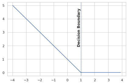
Hinge can be used to create “quasi-SVM” networks, in which the search for a solution that maximizes the separation margin between two class groups is performed. It is defined as [13]:

Where $y,p\in\{-1, 1\}$.

Intuition

This function measures if — and by how much — the proposed margin is being violated by samples that belong to the opposite class. As samples of class -1 and 1 are incorrectly estimated to be of class 1 and -1, respectively, $-yp \gg 0 \implies L_\text{hinge} \gg 0$. The function will also penalize any samples that are correctly classified, but fall under the margin. For example, let $y = -1$ and $p=-0.8$, then

Finally, for any other sample correctly classified with $|p| \ge 1, L_\text{hinge}(y,p) = 0$, and no further gradient updates are performed.

x = tf.reshape(tf.range(-4, 4, delta=.1), (-1, 1))
y = tf.losses.hinge(tf.ones(x.shape), x)

show code

sns.lineplot(x=x.numpy().ravel(), y=y.numpy().ravel())
plt.axvline(1., 0, 5, linestyle=':')
plt.text(1., 2., "Decision Boundary", horizontalalignment='right', weight='semibold', rotation=90)
plt.tight_layout();

Implementation

Hinge loss’ implementation is quite simple, and can be found at keras/losses.py#L1481:

def hinge(y, p):
  if tf.reduce_all((y == 0) | (y == 1)):
    y = 2*y - 1  # convert to (-1, 1)

  return tf.reduce_mean(tf.maximum(1. - y * p, 0.), axis=-1)

Final Considerations

Classification problems are very particular, in the sense that the predicted variable belongs to a very specific, restricted distribution. To this end, we leverage loss functions based on Information Theory principles to train ML models more efficiently and stably.

Notwithstanding, multiple stability and speedup tricks are already implemented in TensorFlow, and can be employed when certain criteria are met. For instance, one can simplify the final activation and loss functions by combining them into a more efficient equation; or select the maximizing outputs of the network instead of multiplying terms that ultimately reduce to zero.

Hopefully, you are now able to better understanding the differences between these functions when training your ML models and transparently select between them.

References

1. J. Han and C. Moraga, “The influence of the sigmoid function parameters on the speed of backpropagation learning,” in International workshop on artificial neural networks, 1995, pp. 195–201.
2. J. Cramer, “The Origins and Development of the Logit Model,” Aug. 2003, doi: 10.1017/CBO9780511615412.010.
3. B. Gao and L. Pavel, “On the properties of the softmax function with application in game theory and reinforcement learning,” arXiv preprint arXiv:1704.00805, 2017.
4. K. Batzner, “Why use softmax as opposed to standard normalization?” Stackoverflow.Available at: https://stackoverflow.com/a/47763299/2429640
5. kmario23, “Numercially stable softmax.” Stackoverflow.Available at: https://stackoverflow.com/a/49212689/2429640
6. Z. Zhang and M. R. Sabuncu, “Generalized cross entropy loss for training deep neural networks with noisy labels,” 2018.
7. C. E. Shannon, “A mathematical theory of communication,” The Bell system technical journal, vol. 27, no. 3, pp. 379–423, 1948.
8. Martı́n Abadi et al., “ TensorFlow: Large-Scale Machine Learning on Heterogeneous Systems.” TensorFlow, 2015.Available at: https://www.tensorflow.org/
9. S. (https://stats.stackexchange.com/users/22311/sycorax), “Should I use a categorical cross-entropy or binary cross-entropy loss for binary predictions?” Cross Validated, 2017.Available at: https://stats.stackexchange.com/q/260537
10. T.-Y. Lin, P. Goyal, R. Girshick, K. He, and P. Dollár, “Focal loss for dense object detection,” in Proceedings of the IEEE international conference on computer vision, 2017, pp. 2980–2988.
11. J. Mukhoti, V. Kulharia, A. Sanyal, S. Golodetz, P. H. S. Torr, and P. K. Dokania, “Calibrating deep neural networks using focal loss,” arXiv preprint arXiv:2002.09437, 2020.
12. S. Humbarwadi, “Object Detection with RetinaNet.” Keras, 2020.Available at: https://keras.io/examples/vision/retinanet/
13. L. Rosasco, E. De Vito, A. Caponnetto, M. Piana, and A. Verri, “Are Loss Functions All the Same?,” Neural computation, vol. 16, pp. 1063–76, Jun. 2004, doi: 10.1162/089976604773135104.