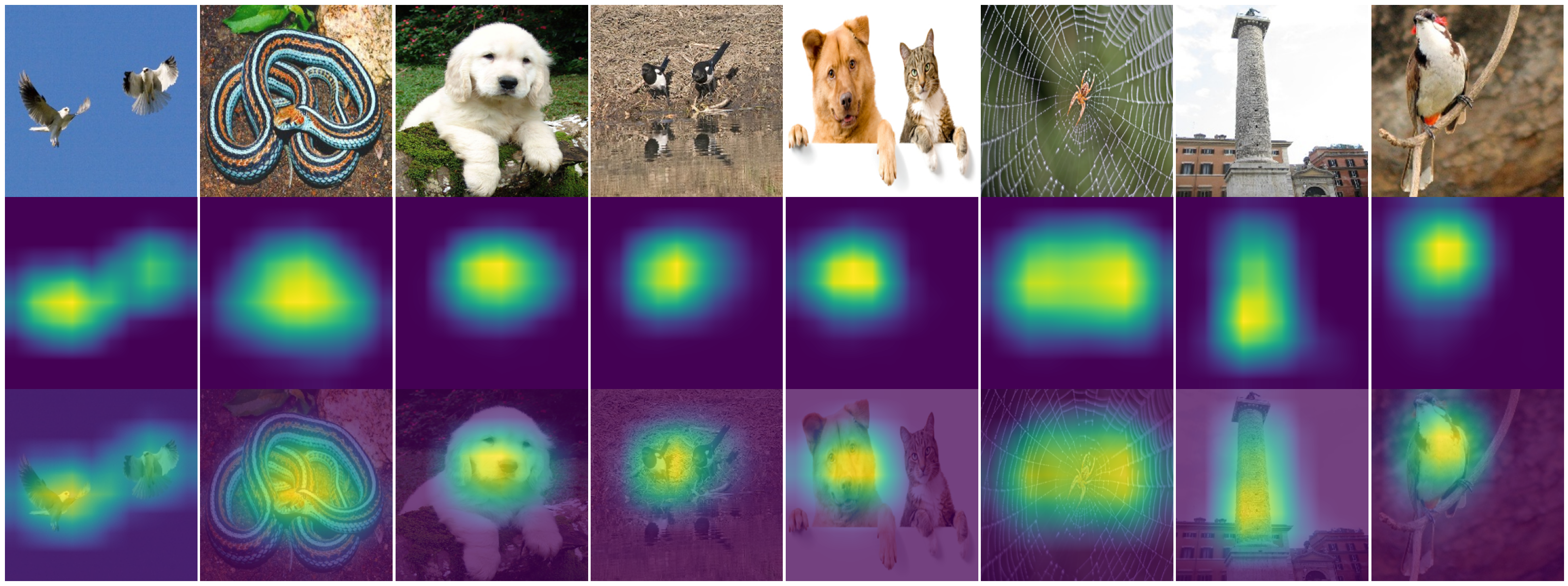
Grad-CAM

This example illustrate how to explain predictions of a Convolutional Neural Network (CNN) using Grad-CAM. This can be easily achieved with the following code template snippet:

import keras_explainable as ke

model = tf.keras.applications.ResNet50V2(...)
model = ke.inspection.expose(model)

scores, cams = ke.gradcam(model, x, y, batch_size=32)

In this page, we describe how to obtain Class Activation Maps (CAMs) from a trained Convolutional Neural Network (CNN) with respect to an input signal (an image, in this case) using the Grad-CAM visualization method. Said maps can be used to explain the model’s predictions, determining regions which most contributed to its effective output.

Grad-CAM is a form of visualizing regions that most contributed to the output of a given logit unit of a neural network, often times associated with the prediction of the occurrence of a class in the problem domain. This method is first described in the following article:

Selvaraju, R. R., Cogswell, M., Das, A., Vedantam, R., Parikh, D., & Batra, D. (2017). Grad-cam: Visual explanations from deep networks via gradient-based localization. In Proceedings of the IEEE international conference on computer vision (pp. 618-626).

Briefly, this can be achieved with the following template snippet:

import keras_explainable as ke

model = build_model(...)
logits, maps = ke.gradients(model, x, y, batch_size=32)

We describe bellow these lines in detail.

Firstly, we employ the Xception network pre-trained over the ImageNet dataset:

model = tf.keras.applications.Xception(
  classifier_activation=None,
  weights='imagenet',
)

print(f'Xception pretrained over ImageNet was loaded.')
print(f"Spatial map sizes: {model.get_layer('avg_pool').input.shape}")

Xception pretrained over ImageNet was loaded.
Spatial map sizes: (None, 10, 10, 2048)

We can feed-forward the samples once and get the predicted classes for each sample. Besides making sure the model is outputting the expected classes, this step is required in order to determine the most activating units in the logits layer, which improves performance of the explaining methods.

from tensorflow.keras.applications.imagenet_utils import preprocess_input

inputs = images / 127.5 - 1
logits = model.predict(inputs, verbose=0)
indices = np.argsort(logits, axis=-1)[:, ::-1]

explaining_units = indices[:, :1]  # First most likely class of each sample.

Grad-CAM works by computing the differential of an activation function, usually associated with the prediction of a given class, with respect to pixels contained in the activation map retrieved from an intermediate convolutional signal (oftentimes advent from the last convolutional layer).

CAM-based methods implemented here expect the model to output both logits and activation signal, so their respective representative tensors are exposed and the jacobian can be computed from the former with respect to the latter. Hence, we modify the current model model — which only output logits at this time — to expose both activation maps and logits signals:

model = ke.inspection.expose(model)
_, cams = ke.gradcam(model, inputs, explaining_units)

ke.utils.visualize(
  images=[*images, *cams, *images],
  overlays=[None] * (2 * len(images)) + [*cams],
)

Note

To increase efficiency, we sub-select only the top \(K\) scoring classification units to explain. The jacobian will only be computed for these \(NK\) outputs.

Following the original Grad-CAM paper, we only consider the positive contributing regions in the creation of the CAMs, crunching negatively contributing and non-related regions together. This is done automatically by ke.gradcam(), which assigns the default value filters.positive_normalize() to the postprocessing parameter.

View page source