Weakly Supervised Object Localization and Semantic Segmentation

Object localization and segmentation cues can be extracted from models trained over multi-label datasets in a weakly supervised setup.

An example of this technique is OC-CSE, which was first described in the paper “Unlocking the potential of ordinary classifier: Class-specific adversarial erasing framework for weakly supervised semantic segmentation.”, by Kweon et al. (2021) [link]. Its original code (written in PyTorch) is available at KAIST-vilab/OC-CSE, but we will actually load its TensorFlow alternative, available at lucasdavid/resnet38d-tf:

COLORS = pascal_voc_colors()
CLASSES = pascal_voc_classes()
WEIGHTS = 'docs/_build/data/resnet38d_voc2012_occse.h5'

! mkdir -p docs/_build/data
! wget -q -nc https://raw.githubusercontent.com/lucasdavid/resnet38d-tf/main/resnet38d.py
! wget -qnc https://github.com/lucasdavid/resnet38d-tf/releases/download/0.0.1/resnet38d_voc2012_occse.h5 -P docs/_build/data/

from resnet38d import ResNet38d

input_tensor = tf.keras.Input(shape=(None, None, 3), name="inputs")
rn38d = ResNet38d(input_tensor=input_tensor, weights=WEIGHTS)

print(f"ResNet38-d with {WEIGHTS} pre-trained weights loaded.")
print(f"Spatial map sizes: {rn38d.get_layer('s5/ac').input.shape}")

! rm resnet38d.py

ResNet38-d with docs/_build/data/resnet38d_voc2012_occse.h5 pre-trained weights loaded.
Spatial map sizes: (None, None, None, 4096)

We can feed-forward the samples once and get the predicted classes for each sample. Besides making sure the model is outputting the expected classes, this step is required in order to determine the most activating units in the logits layer, which improves performance of the explaining methods.

prec = tf.keras.applications.imagenet_utils.preprocess_input

inputs = prec(images.astype("float").copy(), mode='torch')
probs = rn38d.predict(inputs, verbose=0)

Finally, we can simply run all available explaining methods:

rn38d = ke.inspection.expose(rn38d, "s5/ac", 'avg_pool')

# Vanilla CAM
_, cams = ke.cam(rn38d, inputs, batch_size=4)

# TTA-CAM
tta_cam_method = ke.methods.meta.tta(
  ke.methods.cams.cam,
  scales=[0.5, 1.0, 1.5, 2.],
  hflip=True,
)
_, tta_cams = ke.explain(
  tta_cam_method,
  rn38d,
  inputs,
  batch_size=4,
  postprocessing=ke.filters.positive_normalize,
)

Explaining maps can be converted into color maps, respecting the conventional Pascal color mapping:

def cams_to_colors(labels, maps, colors):
  overlays = []
  labels = labels.astype(bool)

  for i in range(8):
    l = labels[i]
    c = colors[l]
    m = maps[i][..., l]
    o = np.einsum('dc,hwd->hwc', c, m).clip(0, 1)
    overlays.append(o)

  return overlays

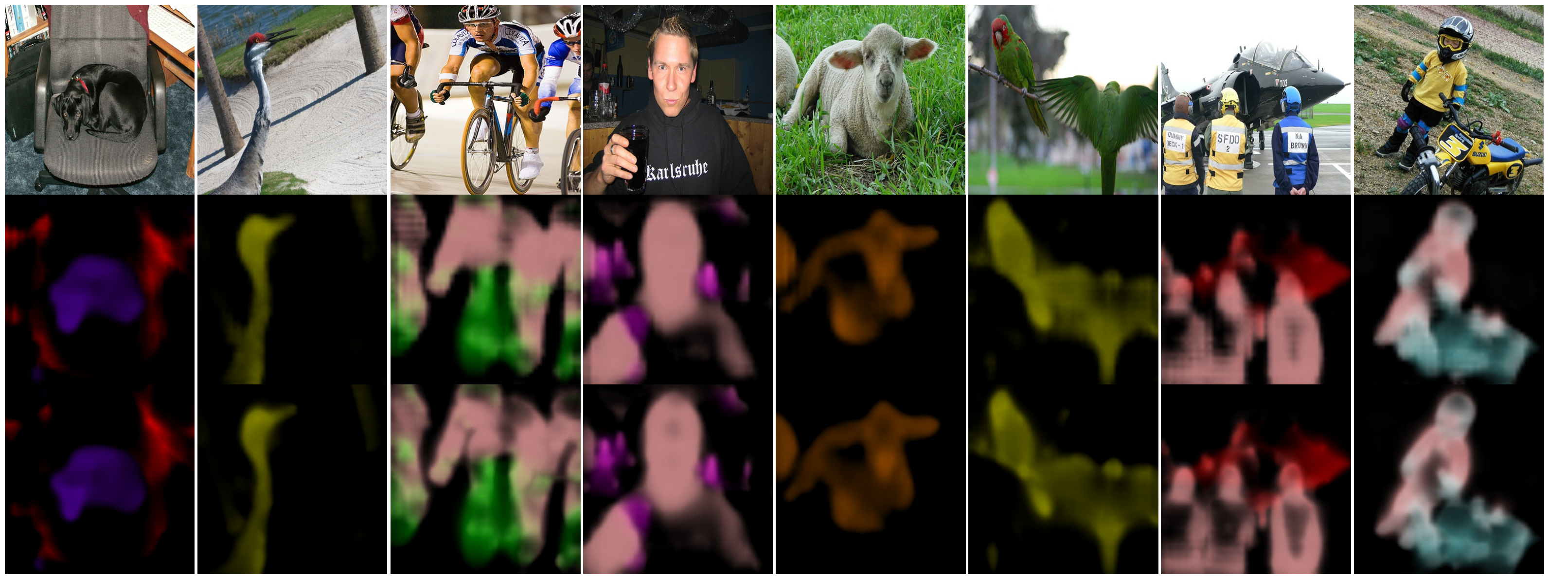
cam_overlays = cams_to_colors(labels, cams, COLORS[1:21])
tta_overlays = cams_to_colors(labels, tta_cams, COLORS[1:21])

ke.utils.visualize([*images, *cam_overlays, *tta_overlays])

View page source