Optimizers and Surfaces

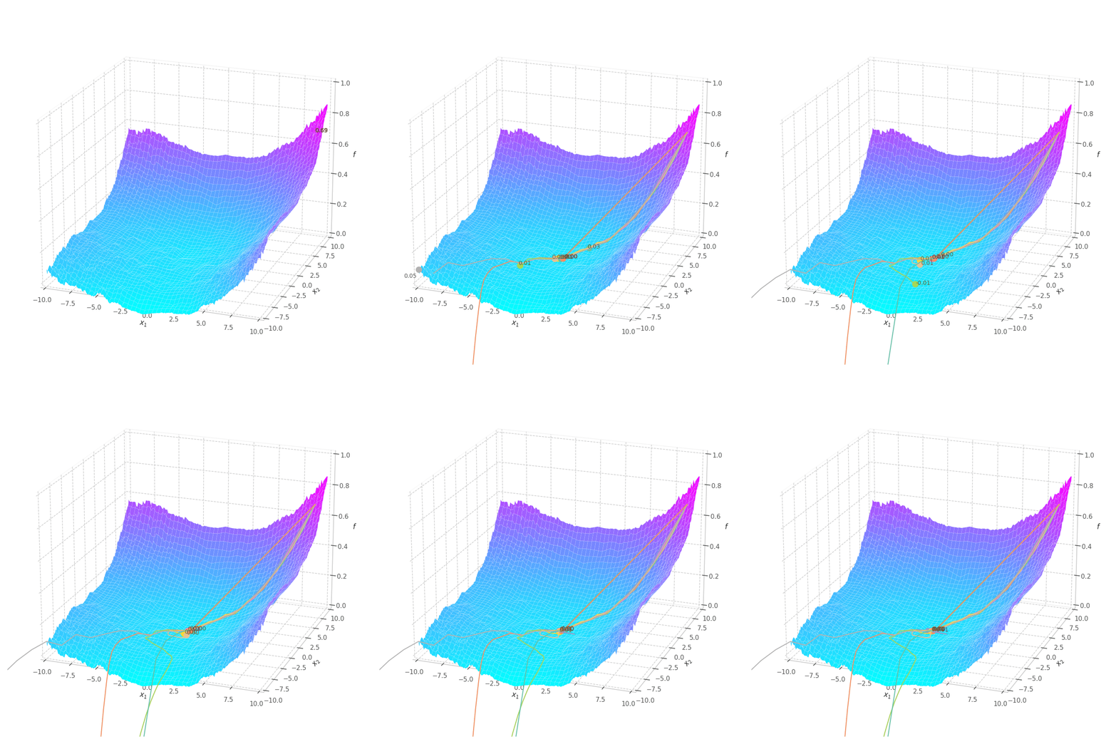
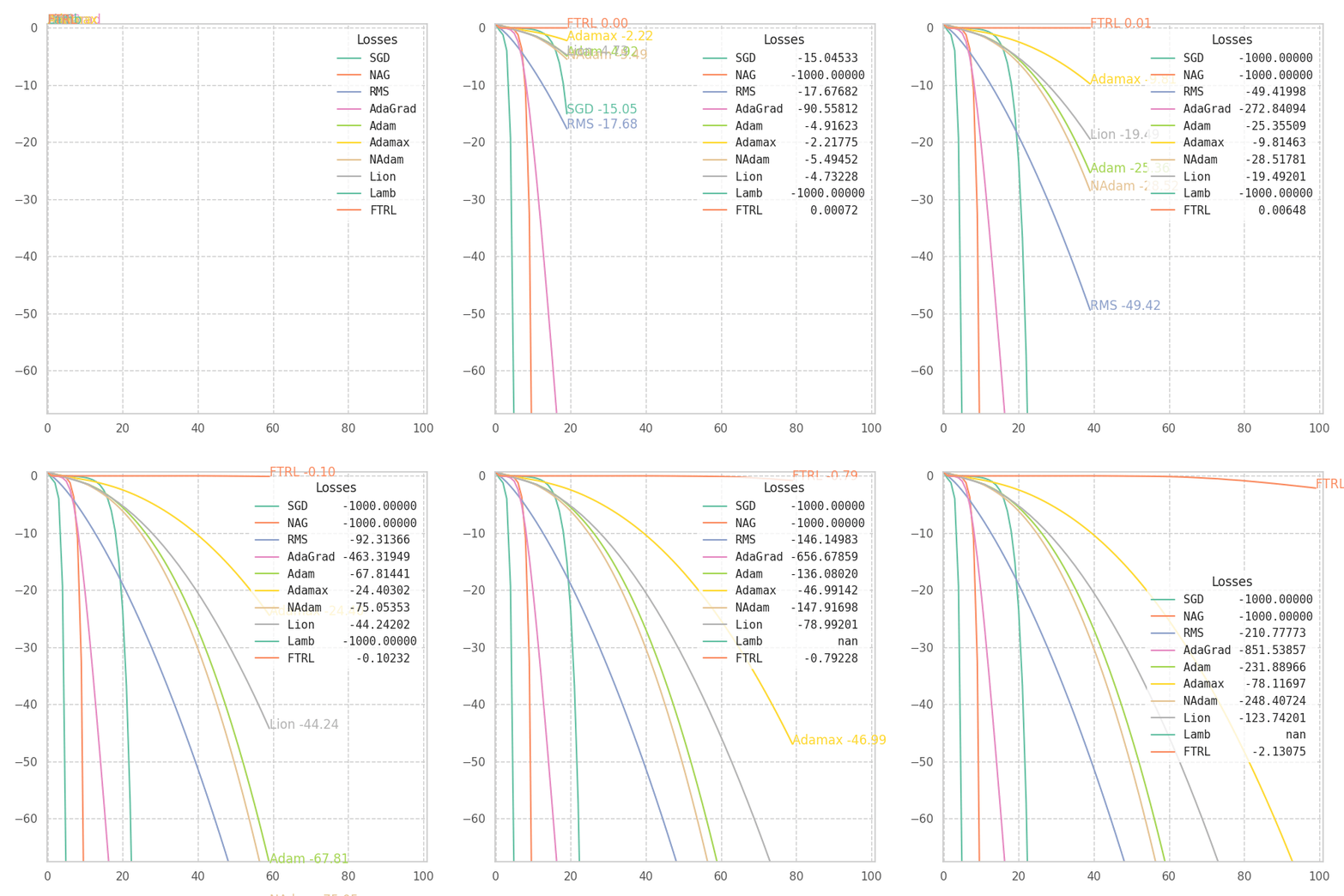
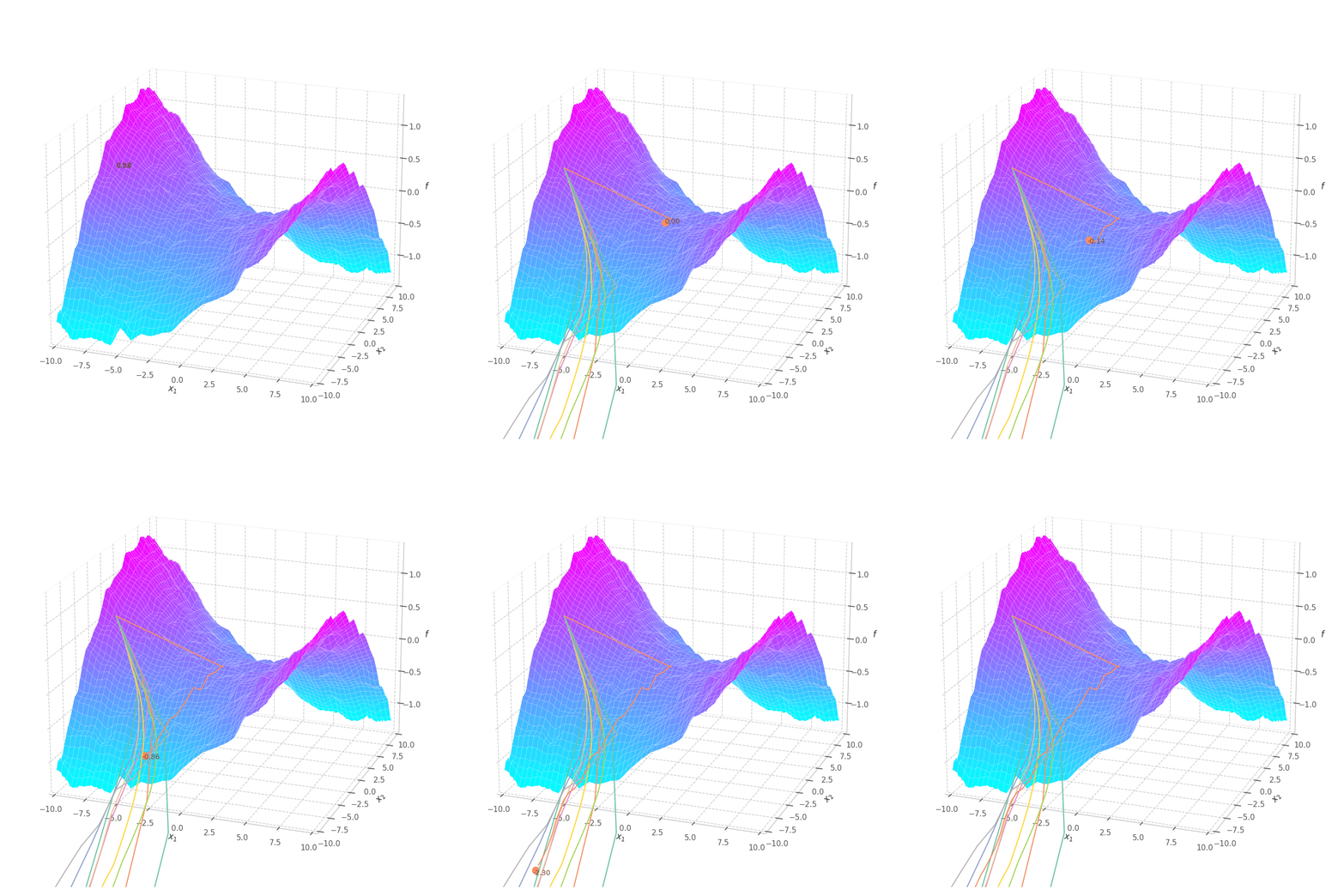
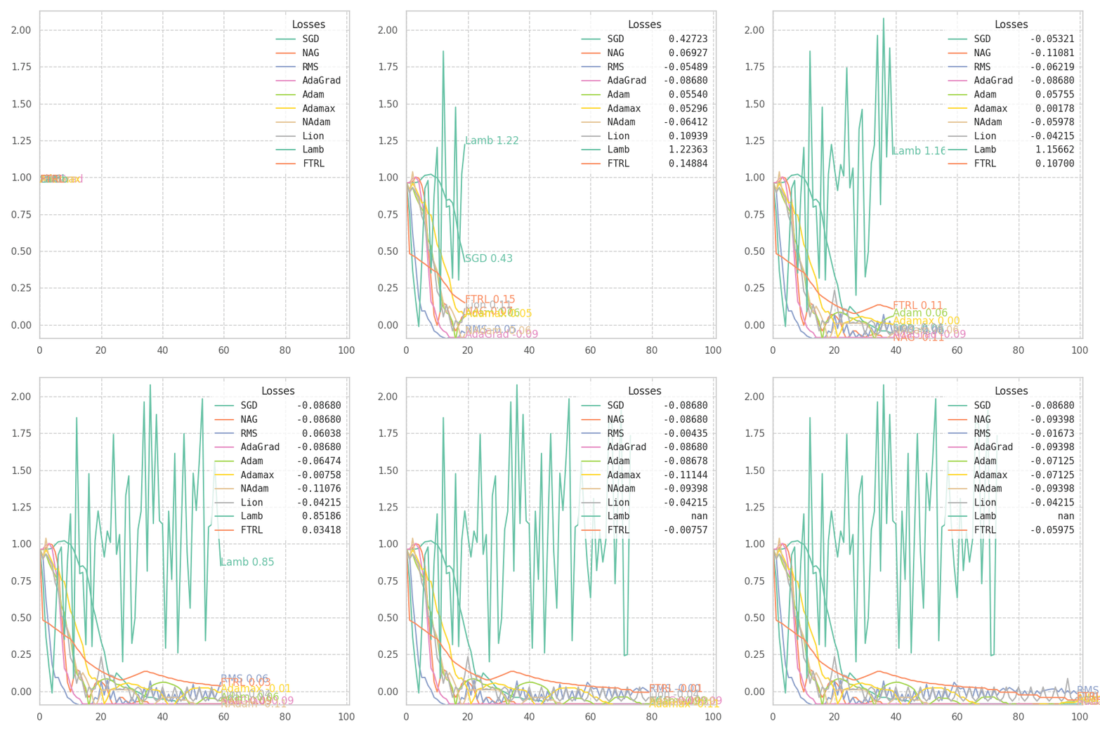
The goal of this post is to give the reader an introduction over the existing optimization algorithms, to illustrate and compare their behavior over the optimization surfaces, which ultimately translates to their effectiveness over AI tasks.

Training a Machine Learning model consists of traverse an optimization surface, seeking the best solution: the configuration of parameters $\bm θ^\star$ associated to the lowest error or best fit. It would be interesting to have a have a visual representation of this process, in which problems such as local minima, noise and overshooting are explicit and better understood.

A Machine Learning model is a parameterized predictive function that associates every input sample to a desired output signal. Formally, let $\bm{x}_i\in \mathbb{R}^f$ be an input sample in the dataset $\mathbf{X} = \lbrace\bm{x}_0, \bm{x}_1, \ldots, \bm{x}_n\rbrace$, then $f(\bm{x}_i,\bm θ_t) = \bm p_i\in\mathbb{R}^c$ is a predictive function parameterized by $\bm θ_t \in \mathbb{R}^m$ at a given training step $t$.

If the problem is supervised, each sample $\bm{x}_i$ is paired with an expected value $\bm{y}_i\in \mathbf{Y}$, often a product of manual and laborious annotation by specialists, and referred to as “ground-truth”. A loss function $\mathcal{L}(\mathbf{X}, \mathbf{Y}, \bm θ_t)$ is also adopted, describing how far off are the predictions outputted by the model parameterized by $\bm θ_t$. Examples of such functions can be checked in my post about cross entropy and logit functions.

As $\bm θ_t$ is contained in the $\mathbb{R}^m$ Euclidean space, it can represented as a point. Moreover, all possible points $\left[\bm θ_t \mid \mathcal{L}(\bm{X}, \bm{Y}, \bm θ_t)\right]$ (obtained by concatenating the parameters with their associated loss values) form a surface in $\mathbb{R}^{m+1}$.

If the functions $f$ and $\mathcal{L}$ are continuously differentiable, then the surface spawned by them is also continuously differentiable. This ensures that the derivative is defined and finite in all points in the domain, and that the Gradient vector can be calculated and used to find the direction of update $-\nabla\mathcal{L}$ for each parameter of the model.

However, many modern models violate this condition by containing non-continuous or non-differentiable functions, such as the Rectified Linear Unit $\text{ReLU}(x) = \max(x, 0)$ function. [1] This isn’t such a big problem, as non-continuous functions employed are always sub-differentiable. I.e., their derivatives can be approximated by known convex functions. As automatic differentiation frameworks (e.g., PyTorch, Tensorflow) often work with pre-defined function and their respective derivatives, non-continuous functions will have one of these convex functions registered as their derivatives.

Model complexity can also severely twist the optimization manifold, resulting in the distancing between the real value and the linear estimation expressed in the gradient. In such cases, it’s common to transverse the search space in smaller steps, reducing the inherit error of optimizing a complex non-linear function through its first order approximation, at the cost of more iterations and higher risk of being stuck at local minima. In practice, however, the optimization surfaces are usually well-behaved (somewhat smooth and simple) if certain conditions are met: [2] the model has few parameters, strong regularization is employed, the underlying function that represents data is also well-behaved.

%config InlineBackend.print_figure_kwargs = {'bbox_inches': None}  # fix for animations with `xlim`.

FIG_SIZES = (9, 9)
VIEW = (30, 70)

XY_RANGE = 10
B = 8

MAX_LOSS_VALUE = 999.99999
MARGIN = 0.05

from IPython.display import HTML
from PIL import Image

import numpy as np
import pandas as pd

import tensorflow as tf

import matplotlib.pyplot as plt
import matplotlib.animation as mpl_animation
import seaborn as sns

sns.set(style='whitegrid')
plt.rcParams.update({'xtick.color':'#555', 'ytick.color':'#555', "animation.embed_limit": 10e9})

plt.rcParams["animation.html"] = "jshtml"


def show_sm_surface(ax, a, b, y, sm=0, title=None, view=(30, 70), cmap=plt.cm.viridis):
  ax.plot_surface(a, b, y[..., sm], cmap=cmap, linewidth=0.1, zorder=1)
  ax.view_init(*view)

  ax.set_xlabel("$x_1$")
  ax.set_ylabel("$x_2$")
  ax.set_zlabel(f"$f$")
  ax.xaxis.pane.fill = False
  ax.yaxis.pane.fill = False
  ax.zaxis.pane.fill = False

  if title: plt.title(title, y=-0.05)
  return ax

def show_surface(x, y, f, ax, view=(20, -70), cmap="cool"):
  ax = show_sm_surface(ax, x, y, f[..., None], sm=0, title='(a)', view=view, cmap=cmap)

  ax.xaxis._axinfo["grid"].update({"linestyle":"--"})
  ax.yaxis._axinfo["grid"].update({"linestyle":"--"})
  ax.zaxis._axinfo["grid"].update({"linestyle":"--"})
  plt.title(None)
  plt.tight_layout()

  return ax


#@title Plotting & Animation Functions

def plot_surface_and_steps(
    opt_points, grads, y, f,
    view=VIEW,
    colors=None,
    title=None,
    zlim="auto",
    duration=1.0,
    legend_title="Optimizers & losses",
    legend=False,
    animated=True,
    figsize=None,
):
  fig = plt.figure(figsize=figsize or FIG_SIZES)
  ax = fig.add_subplot(111, projection = '3d')
  ax = show_surface(z[..., 0], z[..., 1], f, ax, view=view)

  p_point, p_trace, p_texts = {}, {}, {}

  if colors is None:
    colors = list(sns.color_palette("Set2"))
    colors = [colors[i%len(colors)] for i in range(len(opt_points))]
    colors = dict(zip(opt_points, colors))

  p = 1 if animated else None
  last = 0 if animated else -1

  for label, points in opt_points.items():
    c = colors[label]
    c_text = tuple(e/2 for e in c)

    p_point[label] = ax.plot(points[:p, 0], points[:p, 1], y[label][:p], '.', markersize=20, zorder=2, color=c, label=f"{label} {y[label][last]:.5f}")[0]
    p_trace[label] = ax.plot(points[:p, 0], points[:p, 1], y[label][:p], zorder=3, color=c)[0]
    p_texts[label] = ax.text(points[last, 0], points[last, 1], y[label][last], f"{label} {y[label][last]:.2f}", size=10, zorder=4, color=c_text)

  ax.set_xlim((-XY_RANGE, XY_RANGE))
  ax.set_ylim((-XY_RANGE, XY_RANGE))

  if legend:
    L = plt.legend(prop={'family': 'monospace'}, title=legend_title)
  else:
    L = None

  plt.tight_layout()

  # if title: plt.suptitle(title)
  if zlim: ax.set_zlim(zlim)

  if not animated:
    ani = None
  else:
    def _animation_update(num):
      # l_shift = max([t.get_window_extent().width for t in L.get_texts()])
      size = max(len(l) for l in opt_points)

      texts = L.get_texts() if L is not None else [None for _ in opt_points]
      for (label, points), l_text in zip(opt_points.items(), texts):
        if num >= len(points):
          num = len(points)-1

        loss = max(min(y[label][num], MAX_LOSS_VALUE), -MAX_LOSS_VALUE)

        p_point[label].set_data(points[num-1:num, :2].T)
        p_point[label].set_3d_properties(y[label][num-1:num])

        p_texts[label].set_text(f"{loss:.2f}")
        p_texts[label].set_x(points[num, 0]); p_texts[label].set_y(points[num, 1]); p_texts[label].set_z(y[label][num])
        if num > 0:
          p_trace[label].set_data(points[:num-1, :2].T)
          p_trace[label].set_3d_properties(y[label][:num-1])

        if l_text: l_text.set_text(f"{label.ljust(size)} {loss:10.5f}")

    first_points = next(iter(opt_points.values()))
    frames = len(first_points)

    ani = mpl_animation.FuncAnimation(
      fig, _animation_update, frames, interval=duration/frames, blit=False)

  return fig, ax, (p_point, p_trace, p_texts), L, ani


def plot_loss_in_time(y, colors=None, zlim="auto", duration=10000., figsize=None):

  fig = plt.figure(figsize=figsize or FIG_SIZES)
  ax = fig.add_subplot(111)

  p_trace, p_texts = {}, {}

  if colors is None:
    colors = list(sns.color_palette("Set2"))
    colors = [colors[i%len(colors)] for i in range(len(opt_points))]
    colors = dict(zip(opt_points, colors))

  for label, loss in y.items():
    p_trace[label] = plt.plot(loss[:1].clip(-MAX_LOSS_VALUE, MAX_LOSS_VALUE), color=colors[label], label=label)[0]
    p_texts[label] = ax.text(0, loss[:1].clip(-MAX_LOSS_VALUE, MAX_LOSS_VALUE), label, color=colors[label])

  first_points = next(iter(opt_points.values()))
  ax.set_xlim((0-MARGIN, len(first_points)+MARGIN))

  if zlim == "auto":
    all_points = np.concatenate(list(y.values()), 0)
    all_points = all_points[~np.isnan(all_points)]
    zlim = np.quantile(all_points, [0.5, 1.])
    zlim = (zlim[0]-MARGIN, zlim[1]+MARGIN)
  if zlim:
    ax.set_ylim(zlim)

  plt.grid(linestyle="--")
  L = plt.legend(prop={'family': 'monospace'}, title="Losses")
  plt.tight_layout()

  def _animation_update(num):
    label_size = max(len(l) for l in y)

    if num == 0:
      return

    for (label, points), l_text in zip(y.items(), L.get_texts()):
      if num >= len(points):
        num = len(points)-1

      points = np.vstack((
          np.arange(num),
          points[:num].clip(-MAX_LOSS_VALUE, MAX_LOSS_VALUE),
      )).T

      loss = points[-1, 1]
      p_trace[label].set_data(points[:num].T)
      p_texts[label].set_text(f"{label} {loss:.2f}")
      p_texts[label].set_x(points[num-1, 0])
      p_texts[label].set_y(points[num-1, 1])
      l_text.set_text(f"{label.ljust(label_size)} {loss:10.5f}")

  frames = len(first_points)

  ani = mpl_animation.FuncAnimation(
    fig, _animation_update, frames, interval=duration/frames, blit=False)

  return fig, ax, ani

Visualizing Surface Equations

To simulate our problem, we take all points in the 2D mesh grid (-10, 10) (spaced by $0.1$), as well as two noise vectors that simulate fine and coarse-grained noises, respectively:

x = tf.range(-XY_RANGE, XY_RANGE, 0.1, dtype=tf.float32)
x = tf.reshape(x, (-1, 1))
z = tf.stack(tf.meshgrid(x, x), axis=-1)

a, b = z.shape[:2]

r = tf.random.normal((a // B, b // B))
r = tf.image.resize(r[..., None], (a, b), method="bilinear")[..., 0]

c = tf.random.normal((a, b))
c *= tf.abs(z[..., 0]) * tf.abs(z[..., 1]) / 100.0

The vectors c and r contain noise values for each of the $200\times 200$ points in the mesh. However, we can transverse the space and end up in an intermediate location, between two points represented within the mesh. So we also define a approximate_positional_noise function, which determines the noise for a given list of points z by matching these points to their closest neighbors in the mesh:

def approximate_positional_noise(z):
  global r, c

  s = tf.shape(r)
  # Get index (and corresponding noise) for the closest to the input point.
  indices = tf.cast((z+XY_RANGE) * tf.cast(s, tf.float32)/(2*XY_RANGE), tf.int32)
  indices = tf.clip_by_value(indices, 0, s[0] -1)
  return tf.gather_nd(r, indices), tf.gather_nd(c, indices)

Tensorflow stores all operations performed under a tf.GradientTape context, allowing us to automatically compute their Gradient vectors with respect to any variables by simply calling tf.gradient. The direction of highest accent, for a function $f$ and a point $x$, is given by its gradient evaluated at $x$:

@tf.function(reduce_retracing=True)
def compute_grads_scratch(fn, point):
  with tf.GradientTape() as tape:
    x, y = point[..., 0], point[..., 1]
    noise = approximate_positional_noise(point)

    loss = fn(x, y, *noise)
    grad = tape.gradient(loss, point)

  return grad, loss

As our function describes loss or error, optimization is performed by navigating the surface according to the negated gradient. I.e., the direction of highest descent:

def optimize_w_grads(fn, p0, lr, wd, steps=100):
  lr = tf.convert_to_tensor(lr)
  wd = tf.convert_to_tensor(wd)
  point = tf.Variable(p0)

  grads = []
  points = [point.numpy()]

  try:
    for i in range(steps):
      grad, loss = compute_grads_scratch(fn, point)
      point.assign_add(-lr*grad -lr*wd*point)

      grads.append(grad.numpy())
      points.append(point.numpy())
  except Exception as error:
    print(f"Error: {error}")

  grads = np.concatenate(grads, 0)
  points = np.concatenate(points, 0)

  return points, grads

Descriptive Optimization Functions

Now, all that’s left is to define a few optimization functions that will represent our problems:

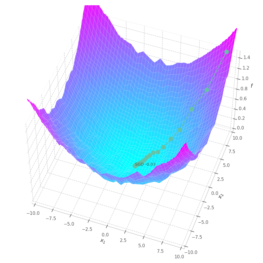
def f0(x, y, r, c):
  # Quadratic Equation Surface ($x^2+y^2$)
  return ((x/10)**2 + (y/10)**2) +0.04*r +0.01*c

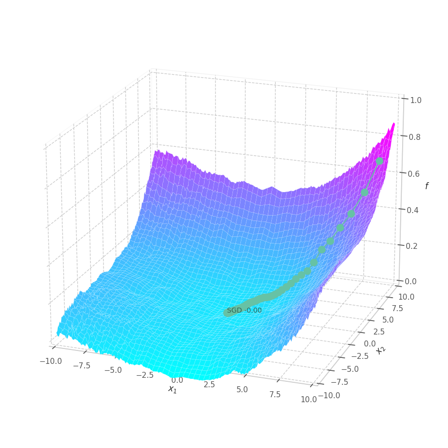
def f1(x, y, r, c):
  # Cubic Equation Surface ($x^3+y^3$)
  return (x**2 + y**2 +0.5*y + 0.06*(x+1)**3 +0.1*(y-1)**3)/400 +0.01*r +0.01*c

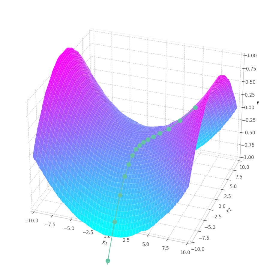
def f2(x, y, r, c):
  # Quadric Equation Surface ($x^2-y^2$)
  return (x**2/2-y**2/2) / 40. +0.01*r +0.01*c

def f3(x, y, r, c):
  # Quadric Equation Surface ($x^2-y^2 -0.75xy$)
  return (x**2/2-y**2/2 -1.5*x*(0.5*y))/60 +0.05*r +0.01*c

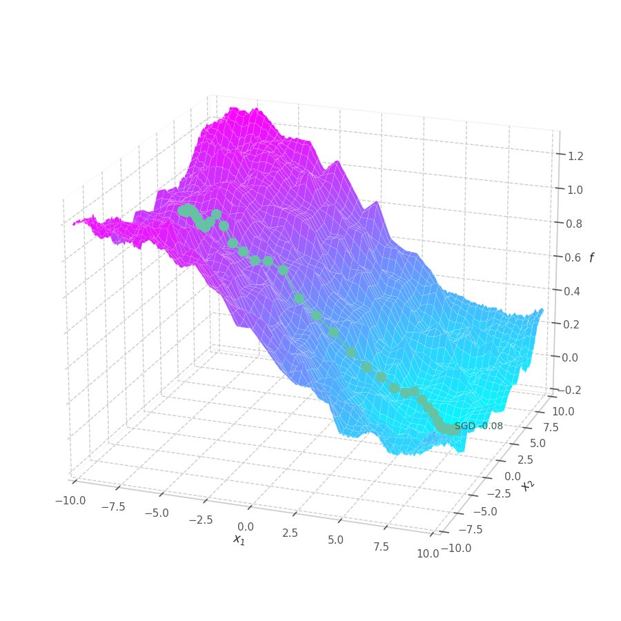
def f4(x, y, r, c):
  # Ramp Equation Surface ($\sin(x/5)-\cos(y/10)$)
  return ((-tf.sin(x/5.) - tf.cos(y/10.))+2)/2 +0.05*r +0.01*c

def f5(x, y, r, c):
  # Elliptic Quadratic Surface ($x/a^2+x/b^2$)
  return ((x/8)**2 + (y/12)**2)/2 +0.04*r +0.01*c

as_opt_set = lambda *x, tag="SGD": ({tag: e} for e in x)

# f0
points, grads = optimize_w_grads(f0, p0=[[9., 9.]], lr=10., wd=0.)
f = f0(z[..., 0], z[..., 1], *approximate_positional_noise(z)).numpy()  # Loss at every grid-point.
y = f0(points[..., 0], points[..., 1], *approximate_positional_noise(points)).numpy()

fig, ax, handlers, L, ani = plot_surface_and_steps(
  *as_opt_set(points, grads, y), f,
  view=(50, -70), zlim=(.0, 1.5), animated=False)
fig.savefig("sgd-s0-quadratic.png")

# f1
points, grads = optimize_w_grads(f1, p0=[[9., 9.]], lr=10., wd=0.)
f = f1(z[..., 0], z[..., 1], *approximate_positional_noise(z)).numpy()  # Loss at every grid-point.
y = f1(points[..., 0], points[..., 1], *approximate_positional_noise(points)).numpy()

fig, ax, handlers, L, ani = plot_surface_and_steps(
  *as_opt_set(points, grads, y), f,
  view=(20, -70), zlim=(.0, 1.), animated=False)
fig.savefig("sgd-s1-cubic.png")

# f2
points, grads = optimize_w_grads(f2, p0=[[7.5, -0.5]], lr=10., wd=0.)
f = f2(z[..., 0], z[..., 1], *approximate_positional_noise(z)).numpy()  # Loss at every grid-point.
y = f2(points[..., 0], points[..., 1], *approximate_positional_noise(points)).numpy()

fig, ax, handlers, L, ani = plot_surface_and_steps(
  *as_opt_set(points, grads, y), f, view=(30, -70), zlim=(-1., 1.), animated=False)
fig.savefig("sgd-s2-quadric.png")

# f3
points, grads = optimize_w_grads(f3, p0=[[-9., 2.5]], lr=10., wd=0.)
f = f3(z[..., 0], z[..., 1], *approximate_positional_noise(z)).numpy()  # Loss at every grid-point.
y = f3(points[..., 0], points[..., 1], *approximate_positional_noise(points)).numpy()

fig, ax, handlers, L, ani = plot_surface_and_steps(
  *as_opt_set(points, grads, y), f, view=(20, -70), zlim=(-1.4, 1.4), animated=False)
fig.savefig("sgd-s3-quadric.png")

# f4
points, grads = optimize_w_grads(f4, p0=[[-7.5, -1.0]], lr=10., wd=0.)
f = f4(z[..., 0], z[..., 1], *approximate_positional_noise(z)).numpy()  # Loss at every grid-point.
y = f4(points[..., 0], points[..., 1], *approximate_positional_noise(points)).numpy()

fig, ax, handlers, L, ani = plot_surface_and_steps(
  *as_opt_set(points, grads, y), f, view=(20, -70), zlim=(-0.2, 1.3), animated=False)
fig.savefig("sgd-s4-ramp.png")

Modern Optimization Methods

Modern optimization strategies are founded on the Gradient-based optimization idea, but often rely on tricks to accelerate or stabilize the walking over the optimization surface. In this section, I introduce some of the optimizers that have recently appeared in literature, detailing their mathematical foundations, and illustrating their optimizing rolling ball over the previously defined surfaces.

Stochastic Gradient Descent

The simplest of the all is called Stochastic Gradient Descent (SGD). [3] In its most known form “mini-batch”, the core idea is to,at each training step $t$, sample the training set for a batch $(\mathbf{X}_t, \mathbf{Y}_t) \subset (\mathbf{X}, \mathbf{Y})$ sufficiently large to closely represent the set, and yet sufficiently small so its gradient computation does not become prohibitive.

As batches may contain some noise, and gradients may not be good estimate for the optimization direction of complex non-linear optimization surfaces, It’s also standard procedure to adopt a learning rate, which can dampen the updates applied to parameters, and, therefore, the mistakes made.

Stochastic Gradient Descent optimization is performed, at a training step $t$, as:

where $x$ is the sample batch, and $\bm θ_{t-1}$ is a vector, containing the model parameters, at step $t-1$. We can visualize how SGD performs, for different learning rates, over a few of the previously defined surfaces:

def get_sgd_with_different_lrs():
  return [
    ("SGD lr: 0.1", tf.optimizers.SGD(learning_rate=0.1)),
    ("SGD lr: 1.0", tf.optimizers.SGD(learning_rate=1.)),
    ("SGD lr:10.0", tf.optimizers.SGD(learning_rate=10.)),
    ("SGD lr:20.0", tf.optimizers.SGD(learning_rate=20.)),
    ("SGD lr:50.0", tf.optimizers.SGD(learning_rate=50.)),
  ]

@tf.function(reduce_retracing=True)
def train_step(fn, point, opt, trainable_vars):
  with tf.GradientTape() as tape:
    x, y = point[..., 0], point[..., 1]
    r, c = approximate_positional_noise(point)

    loss = fn(x, y, r, c)

  grads = tape.gradient(loss, trainable_vars)
  opt.apply_gradients(zip(grads, trainable_vars))

  return grads[0], loss

def optimize_w_opt(fn, optimizer, p0=[[0., 0.]], steps=10):
  point = tf.Variable(p0)
  trainable_vars, points, grads = [point], [point.numpy()], []
  optimizer.build(trainable_vars)

  try:
    for i in range(steps):
      grad, loss = train_step(fn, point, optimizer, trainable_vars)
      grads.append(grad.numpy())
      points.append(point.numpy())
  except Exception as error:
    print(f"Error: {error}")

  return (np.concatenate(points, 0),
          np.concatenate(grads, 0))

def optimize_all_w_opt(fn, opts, p0=[[0., 0.]], steps=100):
  points_and_grads = [optimize_w_opt(fn, opt, p0=p0, steps=steps) for name, opt in opts]
  opt_points = {label: points for (label, _), (points, _) in zip(opts, points_and_grads)}
  opt_grads = {label: grads for (label, _), (_, grads) in zip(opts, points_and_grads)}
  return opt_points, opt_grads

opts = get_sgd_with_different_lrs()
opt_points, opt_grads = optimize_all_w_opt(f0, opts, p0=[[9., 9.]])

f = f0(z[..., 0], z[..., 1], *approximate_positional_noise(z)).numpy()  # Loss at every grid-point.
y = {label: f0(points[..., 0], points[..., 1], *approximate_positional_noise(points)).numpy()
     for label, points in opt_points.items()}

fig, ax, handlers, L, ani = plot_surface_and_steps(
  opt_points, opt_grads, y, f, view=(50, -70), zlim=(.0, 1.5), legend=True)

ani.save("f0-sgd-lr01-50.gif")

opts = get_sgd_with_different_lrs()
opt_points, opt_grads = optimize_all_w_opt(f5, opts, p0=[[9., 9.]])

f = f5(z[..., 0], z[..., 1], *approximate_positional_noise(z)).numpy()  # Loss at every grid-point.
y = {label: f5(points[..., 0], points[..., 1], *approximate_positional_noise(points)).numpy()
     for label, points in opt_points.items()}

fig, ax, handlers, L, ani = plot_surface_and_steps(
  opt_points, opt_grads, y, f, view=(40, -70), zlim=(.0, 1.5), legend=True)
ani.save("f5-sgd-lr01-50.gif")

Our goal is, of course, to reach the best fitted (lowest error) point as quickly as possible. However, the only information available to us relates to a close neighborhood, described by the batch and the current model’s parameters $θ_t$. Gradient Descent must therefore navigate using the vector pointing to the direction of steepest descent (i.e., error decay). This can be seen in the examples above: surface $f_0=x^2+y^2$ is a perfectly circular quadratic function, while $f_5=\frac{x}{8}^2+\frac{y}{12}^2$ is an elliptic surface. A variation in $x$ produces a much higher reduction in $f_5$ (i.e., $f_5(x-\delta, y) < f_5(x, y-\delta)$, for $x\gg 0$), the gradient is steered onto the direction of $x$. Once it becomes sufficiently small, varying $x$ has a marginal overall impact on $f_5$’s value. I.e., the contribution of $x$ to $f_5$ becomes small compared to $y$, reflecting a low derivative value that marginally appears in the gradient. Therefore, the gradient now steers towards the direction that minimizes the second term, $y$.

The biased path taken by SGD has a detrimental effect on training: optimization is slower on elliptic surfaces, where a curved path is taken, and overshooting is more likely to happen for smaller variables. To mitigate this, many solutions employ decomposition methods that project data points onto a representation space in which features are uncorrelated or unrelated. Examples of such methods are: Singular Value Decomposition (SVD), Principal Component Analysis (PCA), [4] and Independent Component Analysis (ICA). [5], [6]

Momentum

One way of bringing more stability to the training procedure is to average gradient vectors, which can build inertia for the update vector, hence steering it onto a more stable direction. [7] To that end, Momentum is a simple extension of SGD that maintains the exponentially decaying average of the update direction, using it to update weights instead:

While highly effective, the accumulation of previous gradient information might inadvertently move weights away from the local minimum point in abrupt changes of the optimization surface’s curvature, occasionally leading to overshooting. Hence, Momentum may benefit from the employment of a decaying learning rate policy.

Nesterov Accelerated Gradient

The Nesterov Accelerated Gradient (NAG), [9] or Nesterov Momentum, is a variation of Momentum design to alleviate overshooting occurrences. It consists of calculating the gradient with respect to the updated data point (i.e., the value we expect it will assume, considering its recent changes), instead of its naive current value.

As $\beta\bm m_{t-1}$ contains the decaying average of the updates committed so far, we expect the parameters to maintain a similar trend. Hence, we define an interim value for parameter $\bm θ_t$:

And define NAG as:

It turns out that it’s not easy to compute $\nabla_θ\mathcal{L}(\mathbf{X}_t, \mathbf{Y}_t, \hat{\bm θ_t})$ without forwarding the signal through the model twice. (Or maybe it could be done by patching the parameters’ values during the forward step?) In any case, Nesterov is more commonly implemented [10] by approximating $\bm m_t$ instead:

Which brings us to NAG’s most common form:

def get_momentum_with_different_lrs():
  return [
    ("NAG lr: 0.1", tf.optimizers.SGD(learning_rate=0.1, momentum=0.9, nesterov=True)),
    ("NAG lr: 1.0",  tf.optimizers.SGD(learning_rate=1.0, momentum=0.9, nesterov=True)),
    ("NAG lr:10.0", tf.optimizers.SGD(learning_rate=10.0, momentum=0.9, nesterov=True)),
    ("NAG lr:20.0", tf.optimizers.SGD(learning_rate=20.0, momentum=0.9, nesterov=True)),
    ("NAG lr:50.0", tf.optimizers.SGD(learning_rate=50.0, momentum=0.9, nesterov=True)),
  ]

opts = get_momentum_with_different_lrs()
opt_points, opt_grads = optimize_all_w_opt(f0, opts, p0=[[9., 9.]])

f = f0(z[..., 0], z[..., 1], *approximate_positional_noise(z)).numpy()  # Loss at every grid-point.
y = {label: f0(points[..., 0], points[..., 1], *approximate_positional_noise(points)).numpy()
     for label, points in opt_points.items()}

fig, ax, handlers, L, ani = plot_surface_and_steps(
  opt_points, opt_grads, y, f, view=(40, -20), zlim=(.0, 1.5), legend=True)

ani.save("f0-Momentum-lr01-50.gif")

opts = get_momentum_with_different_lrs()
opt_points, opt_grads = optimize_all_w_opt(f5, opts, p0=[[9., 9.]])

f = f5(z[..., 0], z[..., 1], *approximate_positional_noise(z)).numpy()  # Loss at every grid-point.
y = {label: f5(points[..., 0], points[..., 1], *approximate_positional_noise(points)).numpy()
     for label, points in opt_points.items()}

fig, ax, handlers, L, ani = plot_surface_and_steps(
  opt_points, opt_grads, y, f, view=(40, -70), zlim=(.0, 1.5), legend=True)
ani.save("f5-momentum-lr01-50.gif")

Momentum converges to close to the global minimum much faster than SGD for both circular and elliptic surfaces, though the later is still slower than the former. All learning rates lead to convergence, although overshooting is more prominent for very large ones. Small values still move at a reasonable pace (through velocity accumulation), making the optimization process more robust to “unreasonable” choices for this hyperparameter.

RMSProb

NAG represents an improvement over SGD in convergence speed, but the difference in weights norms is still noticeable, biasing the gradient towards larger weights, and increasing the risk of overshooting. Going in a different direction, Hinton et al. [11] propose to divide the gradient of each weight by the moving average of its magnitude.

Named RMSprop, the idea behind this method is to normalize changes for each weight, removing the biased gradient directions observed when optimizing with SGD or NAG, and making it invariant to its magnitude throughout training.

For $\rho=0$, the update rule becomes $\bm θ_{t-1} -\eta \frac{\bm g_t}{|\bm g_t|}$. I.e., the sign of the gradient times the learning rate. For larger values, the moving average will roughly point towards a more stable optimization direction, reducing chances of abrupt changes in direction. Furthermore, like gradient clipping, reducing the magnitude of the updates with RMSProp can inadvertently reduce convergence time by damping the effect of noisy batches over updates.

Small variations of the RMSProp algorithm can exist in modern ML libraries. For example, one may consider (a) combining RMSProp with Momentum by defining velocity vectors as decaying average of the amortized gradients (see Adam); or (b) a “centered” version of RMSProp in which the gradient mean is subtracted from moving average of magnitudes, and the gradient is normalized by an estimate of its variance.

def get_rmsprop_with_different_lrs():
  return [
    ("RMS lr:0.100", tf.optimizers.RMSprop(learning_rate=0.01)),
    ("RMS lr:0.025", tf.optimizers.RMSprop(learning_rate=0.025)),
    ("RMS lr:0.05", tf.optimizers.RMSprop(learning_rate=0.05)),
    ("RMS lr:0.075", tf.optimizers.RMSprop(learning_rate=0.075)),
    ("RMS lr:1.0", tf.optimizers.RMSprop(learning_rate=1.0)),
  ]

opts = get_rmsprop_with_different_lrs()
opt_points, opt_grads = optimize_all_w_opt(f0, opts, p0=[[9., 9.]])

f = f0(z[..., 0], z[..., 1], *approximate_positional_noise(z)).numpy()  # Loss at every grid-point.
y = {label: f0(points[..., 0], points[..., 1], *approximate_positional_noise(points)).numpy()
     for label, points in opt_points.items()}

fig, ax, handlers, L, ani = plot_surface_and_steps(
  opt_points, opt_grads, y, f, view=(40, -20), zlim=(.0, 1.5), legend=True)
ani.save("f0-Momentum-lr01-50.gif")

opts = get_rmsprop_with_different_lrs()
opt_points, opt_grads = optimize_all_w_opt(f5, opts, p0=[[9., 9.]])

f = f5(z[..., 0], z[..., 1], *approximate_positional_noise(z)).numpy()  # Loss at every grid-point.
y = {label: f5(points[..., 0], points[..., 1], *approximate_positional_noise(points)).numpy()
     for label, points in opt_points.items()}

fig, ax, handlers, L, ani = plot_surface_and_steps(
  opt_points, opt_grads, y, f, view=(40, -70), zlim=(.0, 1.5), legend=True)
ani.save("f5-momentum-lr01-50.gif")

With SGD and NAG, the step size is not only dictated by the learning rate $\eta$, but also by the norm of the gradient. This implies a bigger updates over points where the optimization surface is steeper, and smaller steps close to local minima. With RMSProp, a constant gradient norm (given a constant learning rate) is observed throughout training, implying a constant update rate. It’s also noticeable that RMSprop moves onto a similar path for both surfaces $f_0$ and $f_5$, mitigating the biased gradient previously observed over elliptic surfaces.

This also implies that progressively reducing the learning rate is paramount for the convergence of the optimization process. This is illustrated in Fig. 11 and Fig. 12, where RMSProp (with learning rate $1.0$) twitches around the $0$ point in later training stages.

AdaGrad

AdaGrad was originally proposed by Duchi et al. in the paper “Adaptive sub-gradient methods for online learning and stochastic optimization”. [12] The authors give a great introduction over it:

We present a new family of sub-gradient methods that dynamically incorporate knowledge of the geometry of the data observed in earlier iterations to perform more informative gradient-based learning. Metaphorically, the adaptation allows us to find needles in haystacks in the form of very predictive but rarely seen features. Our paradigm stems from recent advances in stochastic optimization and online learning which employ proximal functions to control the gradient steps of the algorithm. — Duchi et al. [12]

The “geometry of the data” is represented by the mutual change in the components of the Gradient over the optimization surface. Formally, AdaGrad updates weights according to the following rule.

where $\bm G_t$ contains the sum of the outer products of all previous gradient vectors with themselves, and $\bm G_t^{-1/2}$ is the inverse of the square root of matrix $\bm G_t$.

Multiplying $\bm G_t^{-1/2}$ by $\bm g_{t}$ projects the gradient onto a normalized vector space where the difference between its components is smaller, as the change rate $\bm g_{t,i}$ of each parameter $i$ is scaled by the inverse of the sum of its absolute mutual change with every other parameter. Parameters with strong variation will have their update rate dampened, approximating them to the change rate of the “comparatively rare features.” [12]

However, the time complexity required to compute the root square and the matrix inversion $\bm G_{t}^{-1/2}$ is $O(n^2)$, implying higher computational footprint and much longer training times than the previous optimizers. A simpler and less computationally intensive alternative is thus implemented by most machine learning frameworks.

This “simpler” alternative only uses the main diagonal of $\bm G_t$, invariably assuming that the remaining elements of the matrix are close to zero. That is, that most of the variation observed is concentrated in the components’ second moments ($\bm G_{t,i,i}=\bm g_{t,i}^2 \gg 0$), and that these components become somewhat linearly independent over time ($\bm G_{t,i,j} \approx 0$, for $i\neq j$):

where $\odot$ is the Hadamard product (element-wise multiplication).

Observing Changes Made by AdaGrad

We can visualize what AdaGrad is doing by sampling un-normalized “gradients” from a random distribution and computing their associated $\bm G_t^{-1/2}$:

from scipy import linalg

def adagrad_w_full_gt(n=3, f=2, scales=(1.0, 2.0), random_state=None):
  Gt = 0
  for t in range(n):
    gt = random_state.rand(f) * scales
    Gt += np.outer(gt, gt)
    Gt_inv = linalg.inv(linalg.sqrtm(Gt) + np.eye(len(Gt))*1e-5)
    vt = (Gt_inv @ gt[..., np.newaxis]).ravel()
    yield gt, vt

def adagrad_w_diag_gt(n=3, f=2, scales=(1.0, 2.0), random_state=None):
  Gt = 0
  for t in range(n):
    gt = random_state.rand(f) * scales
    Gt += gt**2
    vt = gt / (np.sqrt(Gt)+1e-5)
    yield gt, vt

N = 8
F = 2
SCALES = (0.5, 2.0)
SEED_1 = np.random.RandomState(32)
SEED_2 = np.random.RandomState(53)

def plot_adagrads(grads, n=10, xlim=(-1, 1), ylim=(0, 1)):
  plt.figure(figsize=(9, 9))

  for t, (gt, vt) in enumerate(grads):
    xytext = [0.02, -0.02]
    a_u = N/2
    alpha = min(1.0*(t+1-a_u)**2/a_u**2 + 0.1, 1.0)
    ax = plt.arrow(0, 0, gt[0], gt[1], color='gray', head_width=0.02, head_length=0.03, alpha=alpha)
    ax = plt.arrow(0, 0, vt[0], vt[1], color='teal', head_width=0.02, head_length=0.03, alpha=alpha)
    plt.annotate(f"$\|g_{t}\| = {linalg.norm(gt):.1f}$", xy=gt, xytext=gt+xytext, color='gray', alpha=alpha)
    plt.annotate(f"$\|v_{t}\| = {linalg.norm(vt):.1f}$", xy=vt, xytext=vt+xytext, color='teal', alpha=alpha)

  plt.xlim(xlim)
  plt.ylim(ylim)
  plt.tight_layout()

plot_adagrads(adagrad_w_full_gt(n=N, f=F, scales=SCALES, random_state=SEED_1), n=N, ylim=(0, 2))
plot_adagrads(adagrad_w_diag_gt(n=N, f=F, scales=SCALES, random_state=SEED_2), n=N, xlim=(0, 1.2), ylim=(0, 1.2))

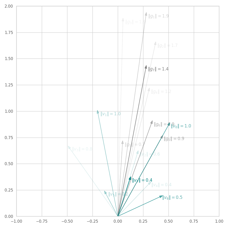
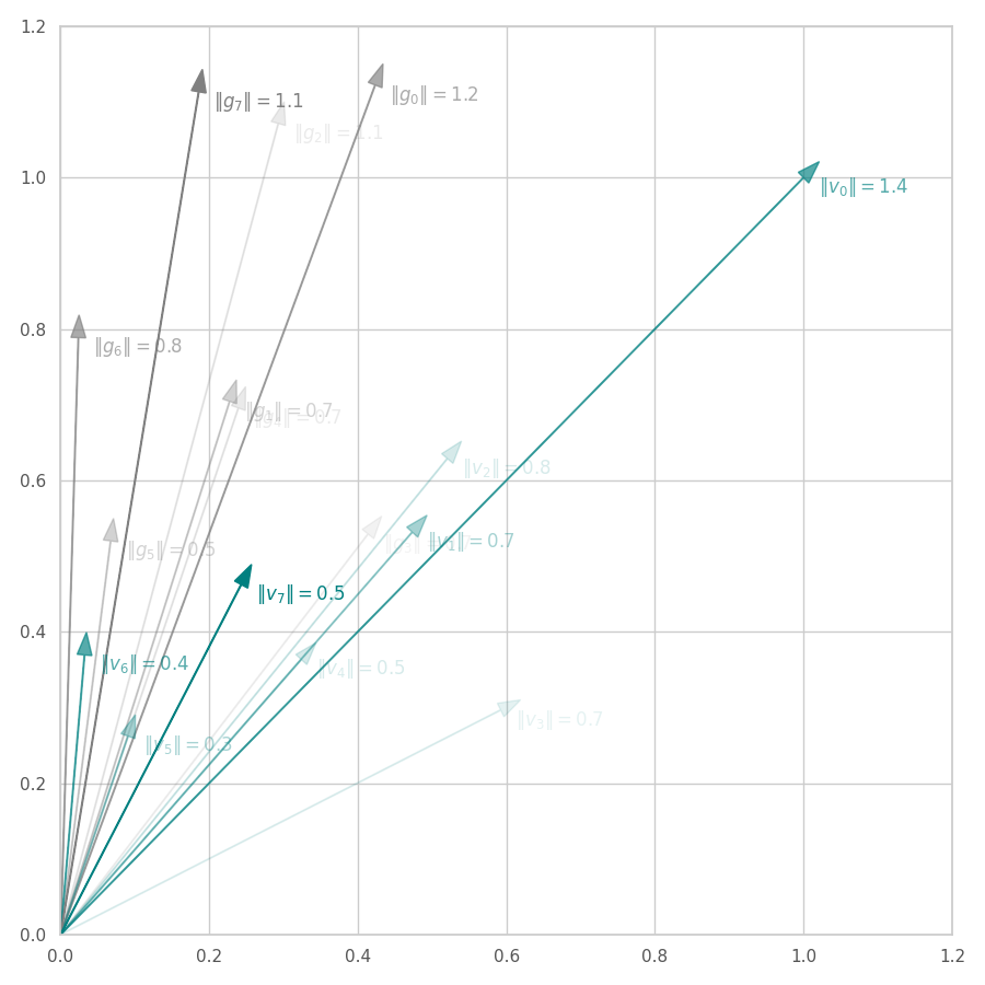
From the Figures above, we observe that:

• AdaGrad “full” version. As seen in Fig. 13, $\bm g_0$ is scaled down to $\bm v_0$, resulting in normalized change directions ($|\bm v_0| = 1$). Subsequent steps maintain a lower normed update direction $\bm v_t$ by dampening the $y$ component in favor of the $x$ one. As $t$ increases, we expect $\bm g_t$ (and $\bm v_t$) to become smaller due to $\bm θ_t$ being closer to local minima and the accumulation of $\bm G_t$. Eventually, $\bm g_t$ should approximate to $0$, implying in the convergence of $\bm G_t$ and of the training procedure (check the training illustrated in the optimization surface bellow).

• AdaGrad “diagonal” version. With AdaGrad’s alternative implementation, illustrated in Fig. 14, the first gradient $\bm v_0$ is scaled down to have its individual components equal to $1$. This process produces a biased update vector, as its direction is slightly changed. Hence, $||\bm v_0|| = \sqrt{2} \approx 1.4$. Following iterations of AdaGrad approximate $||\bm v_t||$ to zero. Like in the full version, the update direction is amortized over time.

N = 8
F = 1024
SCALES = np.random.lognormal(size=F)
SEED_1 = np.random.RandomState(32)
SEED_2 = np.random.RandomState(53)

%timeit list(adagrad_w_full_gt(n=N, f=F, scales=SCALES, random_state=SEED_1))
%timeit list(adagrad_w_diag_gt(n=N, f=F, scales=SCALES, random_state=SEED_2))

27.4 s ± 1.86 s per loop (mean ± std. dev. of 7 runs, 1 loop each)
619 µs ± 162 µs per loop (mean ± std. dev. of 7 runs, 1000 loops each)

def get_adagrad_with_different_lrs():
  return [
    ("AdaG lr: 0.01", tf.optimizers.Adagrad(learning_rate=0.01)),
    ("AdaG lr: 0.10", tf.optimizers.Adagrad(learning_rate=0.1)),
    ("AdaG lr: 0.50", tf.optimizers.Adagrad(learning_rate=0.5)),
    ("AdaG lr: 1.00", tf.optimizers.Adagrad(learning_rate=1.0)),
    ("AdaG lr:10.00", tf.optimizers.Adagrad(learning_rate=10.0)),
  ]

#@title $f_0$ - AdaGrad
opts = get_adagrad_with_different_lrs()
opt_points, opt_grads = optimize_all_w_opt(f0, opts, p0=[[9., 9.]])
f = f0(z[..., 0], z[..., 1], *positional_noise(z)).numpy()  # Loss at every grid-point.
y = {label: f0(points[..., 0], points[..., 1], *positional_noise(points)).numpy()
     for label, points in opt_points.items()}
fig, ax, handlers, L, ani = plot_surface_and_steps(
  opt_points, opt_grads, y, f, view=(50, -70), zlim=(.0, 1.5), legend=True)
ani.save("f0-adagrad-lr-0001-10.gif")

#@title $f_5$ - AdaGrad
opts = get_adagrad_with_different_lrs()
opt_points, opt_grads = optimize_all_w_opt(f5, opts, p0=[[9., 9.]])
f = f5(z[..., 0], z[..., 1], *positional_noise(z)).numpy()  # Loss at every grid-point.
y = {label: f5(points[..., 0], points[..., 1], *positional_noise(points)).numpy()
     for label, points in opt_points.items()}
fig, ax, handlers, L, ani = plot_surface_and_steps(
  opt_points, opt_grads, y, f, view=(40, -70), zlim=(.0, 1.5), legend=True)
ani.save("f5-adam-lr0001-10.gif")

#@title $f_4$ - AdaGrad
opts = get_adagrad_with_different_lrs()
opt_points, opt_grads = optimize_all_w_opt(f4, opts, p0=[[-7.5, -1.0]])
f = f4(z[..., 0], z[..., 1], *positional_noise(z)).numpy()  # Loss at every grid-point.
y = {label: f4(points[..., 0], points[..., 1], *positional_noise(points)).numpy()
     for label, points in opt_points.items()}
fig, ax, handlers, L, ani = plot_surface_and_steps(
  opt_points, opt_grads, y, f, view=(20, -70), zlim=(-0.2, 1.3), legend=True)
ani.save("f4-adam-lr0001-10.gif")

While the constant accumulation of $\bm G_t$ assures convergence, it can inadvertently cause a problem: as $\bm G_t$ can become relatively large at early steps, the gradients might be nullified, implying early convergence and an underfit solution. This is seen in Fig. 16, where many choice of learning rate cause AdaGrad to get stuck at local minima.

AdaDelta is a direct extension of AdaGrad that aims to overcome the aforementioned limitation by setting a decay rate $\rho\in[0, 1]$, and maintaining the Exponential Moving Average (EMA) of the past squared gradients and squared updates. RMSProp is identical to AdaDelta if the squared updates were discarded. [13]

Adam

Adam is one of the most popular optimization algorithms nowadays. Its name stands for “adaptive moment estimation”, [14] and consists of keeping track the moving average for the first and second moments (just like Momentum and RMSprop, respectively), and using them to regularize the direction of update of the weights.

Formally, Adam is defined as:

where $\beta_1$ and $\beta_2$ are hyperparameters similar to Momentum’s $\beta$ and RMSProp’s $\rho$, respectively, and $\beta^t$ represents the hyperparameters $\beta$ to the power $t$. These frequently assume high values (such as 0.9 and 0.999), indicating its preference for retaining a long Gradient footprint throughout training.

Adam’s most noticeable difference to previous methods are the correction terms $1/(1-\beta^t_1)$ and $1/(1-\beta^t_2)$, which are employed to counter-weight the initial bias of the terms $\bm m_t$ and $\bm v_t$ towards $0$, specially when $\beta_1$ and $\beta_2$ terms are very large. [14] Notice that, for $t=1$ (first training step), $\hat{\bm m_t} = \bm g_t$ and $\hat{\bm v_t} = \bm g_t^2$. For a large $t$ (once many steps are taken), $\beta^t_1, \beta^t_2 \to 0$, hence $\hat{\bm m_t} \to \bm m_t$ and $\hat{\bm v_t} \to \bm v_t$.

def get_adam_with_different_lrs():
  return [
    ("Adam lr: 0.001", tf.optimizers.Adam(learning_rate=0.001)),
    ("Adam lr: 0.01", tf.optimizers.Adam(learning_rate=0.01)),
    ("Adam lr: 0.1", tf.optimizers.Adam(learning_rate=0.1)),
    ("Adam lr: 1.0",  tf.optimizers.Adam(learning_rate=1.0)),
    ("Adam lr:10.0", tf.optimizers.Adam(learning_rate=10.0)),
  ]

#@title $f_5$ - Adam
opts = get_adam_with_different_lrs()
opt_points, opt_grads = optimize_all_w_opt(f5, opts, p0=[[9., 9.]])
f = f5(z[..., 0], z[..., 1], *positional_noise(z)).numpy()  # Loss at every grid-point.
y = {label: f5(points[..., 0], points[..., 1], *positional_noise(points)).numpy()
     for label, points in opt_points.items()}
fig, ax, handlers, L, ani = plot_surface_and_steps(
  opt_points, opt_grads, y, f, view=(40, -70), zlim=(.0, 1.5), legend=True)
ani.save("f5-adam-lr0001-10.gif")

#@title $f_4$ - Adam
opts = get_adam_with_different_lrs()
opt_points, opt_grads = optimize_all_w_opt(f4, opts, p0=[[-7.5, -1.0]])
f = f4(z[..., 0], z[..., 1], *positional_noise(z)).numpy()  # Loss at every grid-point.
y = {label: f4(points[..., 0], points[..., 1], *positional_noise(points)).numpy()
     for label, points in opt_points.items()}
fig, ax, handlers, L, ani = plot_surface_and_steps(
  opt_points, opt_grads, y, f, view=(20, -70), zlim=(-0.2, 1.3), legend=True)
ani.save("f4-adam-lr0001-10.gif")

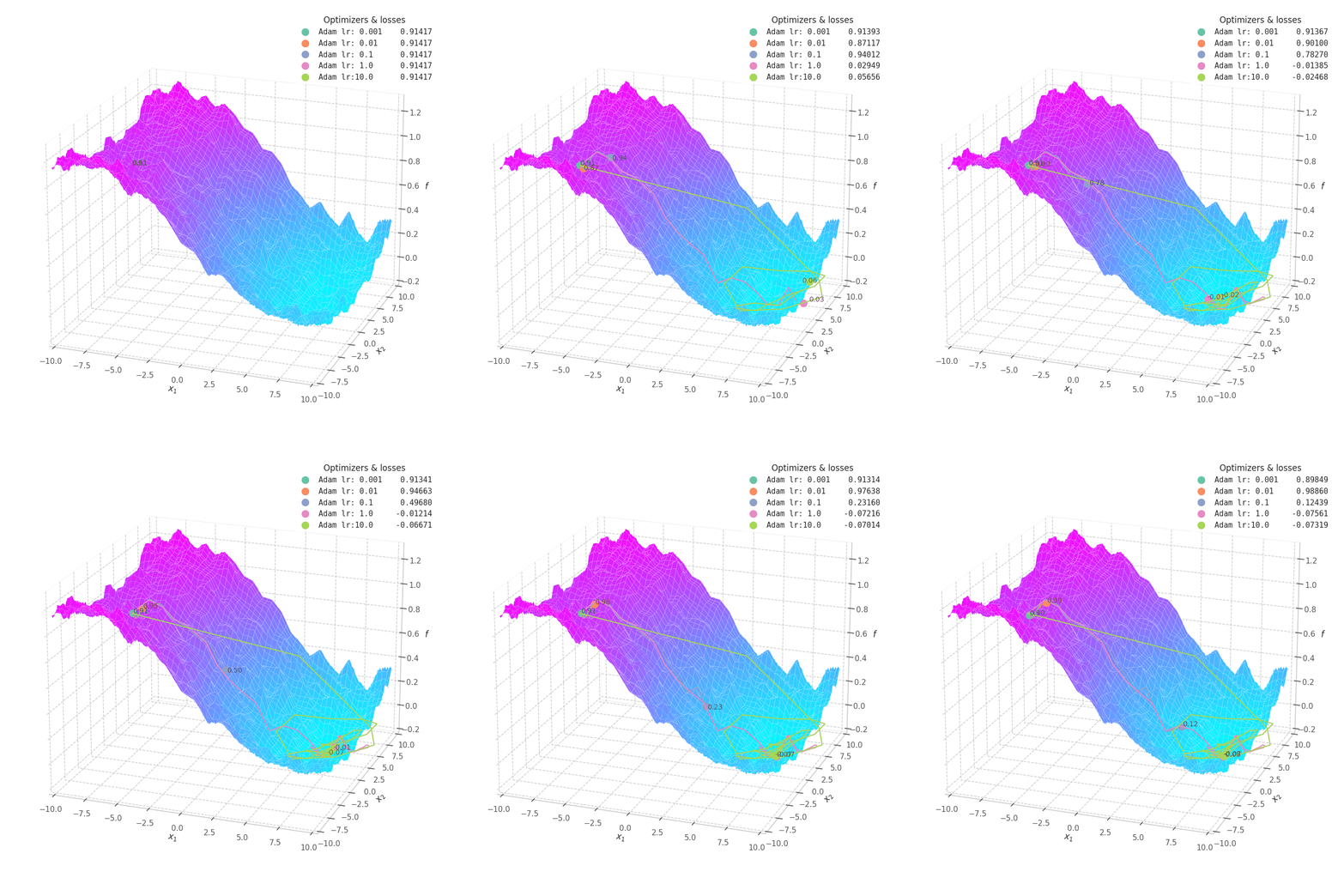
Firstly, Adam converges much faster than RMSprop (due to gradient first moment accumulation), while many choices for the learning rate (between $0.01$ and $10$) seem to work for the noisy ramp ($f_4$) and elliptic ($f_5$) surfaces. Adam is considered fairly robust to changes of hyperparameters. [15]

Less twitching — compared with RMSProp — is also observed at later training steps, when the optimizing surface becomes flatter and the accumulated $\bm m_t$ becomes small. Conversely, we can also see the solution getting stuck in local minima points when tiny learning rates are employed to transverse noisy optimization surfaces (e.g., $f_5$).

Adam also has many variations. One of these is AdaMax, also defined by Kingma et al. [14], in which $\bm v_t$ is defined as $\max(\beta_2 \bm v_{t-1}, |\bm g_t|)$ (i.e., the $L^\infty$ norm of the gradient). Another variation is NAdam, [16], which can be loosely seen as “RMSprop with Nesterov momentum”. All of these formulations are commonly implemented in modern machine learning frameworks: tf/Adam, tf/AdaMax, tf/NAdam, torch/Adam, torch/AdaMax, and torch/NAdam.

Lion

In 2023, Chen et al. [17] proposed an algorithm to perform program search. In it, an “infinite and sparse program space” is searched after an optimization method that is both effective and memory-efficient. Starting from an initial program (AdamW), the search algorithm results is the Lion (Evolved Sign Momentum) optimizer, one of the first optimization methods devised with the assist of machine learning.

Lion is defined as:

where $\beta_1=0.9$ and $\beta_2=0.99$ by default.

Lion is similar to Adam and RMSprop, in which the gradient is accumulated and normalized. However, it is more memory-efficient than Adam, as it does not rely on the second-order moment to normalize the magnitude of the update step. It is also reasonable to assume that the learning rate should be smaller than Adam’s, considering that the sign function should produce an update vector with higher norm. Of course, like RMSprop, scheduling the reduction of learning rate is important to assure convergence at later stages of training.

def get_lion_with_different_lrs():
  return [
    ("Lion lr:0.01", tf.optimizers.Lion(learning_rate=0.01)),
    ("Lion lr:0.1", tf.optimizers.Lion(learning_rate=0.10)),
    ("Lion lr:0.25", tf.optimizers.Lion(learning_rate=0.25)),
    ("Lion lr:0.5", tf.optimizers.Lion(learning_rate=0.50)),
    ("Lion lr:1.0", tf.optimizers.Lion(learning_rate=1.00)),
  ]

#@title $f_5$ - Lion
opts = get_lion_with_different_lrs()
opt_points, opt_grads = optimize_all_w_opt(f5, opts, p0=[[9., 9.]])
f = f5(z[..., 0], z[..., 1], *positional_noise(z)).numpy()  # Loss at every grid-point.
y = {label: f5(points[..., 0], points[..., 1], *positional_noise(points)).numpy()
     for label, points in opt_points.items()}
fig, ax, handlers, L, ani = plot_surface_and_steps(
  opt_points, opt_grads, y, f, view=(40, -70), zlim=(.0, 1.5), legend=True)
ani.save("f5-lion-lr05-1.gif")

#@title $f_4$ - Lion
opts = get_lion_with_different_lrs()
opt_points, opt_grads = optimize_all_w_opt(f4, opts, p0=[[-7.5, -1.0]])
f = f4(z[..., 0], z[..., 1], *positional_noise(z)).numpy()  # Loss at every grid-point.
y = {label: f4(points[..., 0], points[..., 1], *positional_noise(points)).numpy()
     for label, points in opt_points.items()}
fig, ax, handlers, L, ani = plot_surface_and_steps(
  opt_points, opt_grads, y, f, view=(20, -70), zlim=(-0.2, 1.3), legend=True)
ani.save("f4-lion-lr05-1.gif")

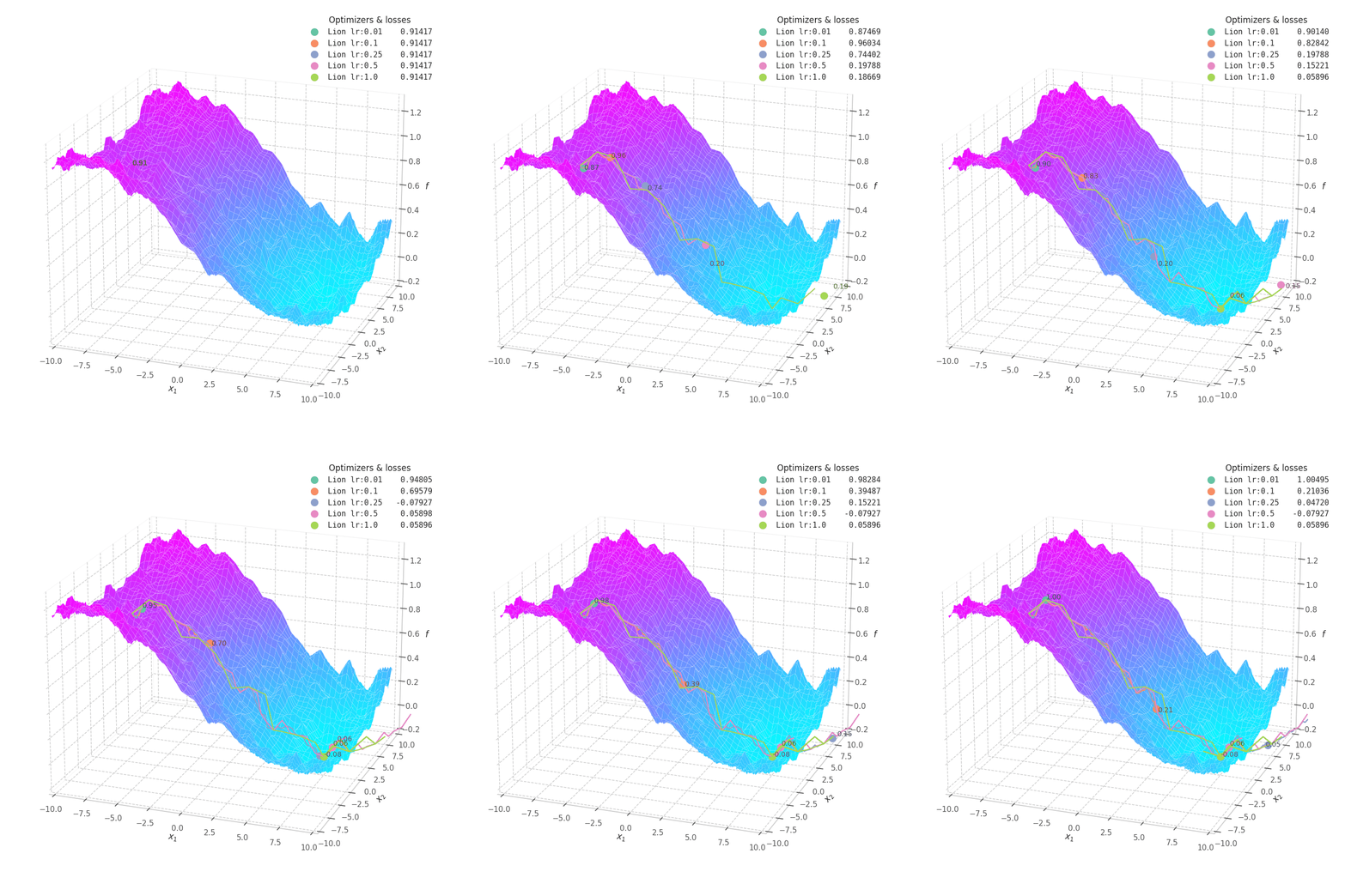
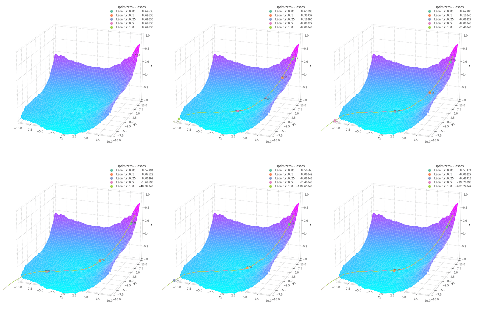
Lion is much more sensible to a choice of learning rate, becoming highly unstable and resulting in overshooting for large values. On the other hand, small values produce slower (but steady) progress towards local minima, while still being robust against bumps in a noisy optimization surface.

Even though momentum can still be accumulated in steep regions of the optimization space, Lion will converge slower than Adam due to the restrictive constraint applied to the update step (the sign function). We also observe twitching at later stages of training over surfaces with easily found minimum points ($f_4$ and $f_5$), when employing a constant learning rate.

LARS & LAMB

While the previous methods are the most popular choices for daily tasks, achieving fast convergence for many problems and reasonable batch sizes (higher than 8 and lower than 8,192), one may wish to increase batch size even further, given compatible hardware is available. Huge batch sizes allow us to present the entire dataset in the model’s training loop in just a few steps, which could greatly reduce training time.

However, simply increasing the batch size tends to have a negative impact on accuracy, as (a) fewer steps will be taken, each still limited by the learning rate; and (b) a large quantity of samples (associated with many different tasks) may result in strong coefficients from a great number of features, adding strong noise to the gradient. Therefore, naively increasing batch can result in a sub-optimal training.

A common practice is “linear LR scaling”: to increase learning rate proportionally to the batch size, [18] thus accounting for the increase in stability and reduction in number of steps, but even that has a limit: using SGD, AlexNet and ResNet-50 cannot learn the ImageNet dataset with batches larger than 1,024 and 8,192 samples, respectively. In practice, increasing both learning rate and batch size above a number (such as 512) is troublesome, as training becomes unstable due to noise injected by exaggerated gradients devised from noisy batches and large learning rates.

LARS

While a range of techniques were devised to improve upon this limit (such as scheduling an increasing learning rate at early training stages), one quickly gained notoriety in the Literature: Layer-wise Adaptive Rate Scaling (LARS) [19] is an (per-weight) adaptive strategy that comprises calculating the ratio between the $L_2$-norms of the weight and its Gradient.

If LR is large comparing to the ratio for some layer, then training may becomes unstable. The LR “warm-up” attempts to overcome this difficulty by starting from small LR, which can be safely used for all layers, and then slowly increasing it until weights will grow up enough to use larger LRs. We would like to use different approach. We use local LR $\bm λ_l$ for each layer $l$. — You et al. [19]

LARS redefines the update delta in SGD by considering a “local LR” $\bm λ^l$ for each layer $l$, comprising parameters $\bm θ_t^l \subset \bm θ_t$:

where $γ_t$ is a scheduling factor for the learning rate, and $\eta$ is the LARS coefficient: a “local” learning rate base value used to express our confidence in $\bm λ^l$.

Intuitively, LARS’s normalized update vector $\bm g_t / ||\bm g_t||_2$ becomes independent to the magnitude of the Gradient, while still being compatible with the weight norm, hence mitigating the exploding and vanishing gradient problems. The step size will increase proportional to the parameter’s norm, as large parameters are expected to be associated with large (and yet meaningful) Gradients.

The authors further consider the effect of weight decay on the update direction, as well as momentum, when computing $\bm λ_t$:

You et al. successfully trained models with batch sizes as large as 32k, without displaying expressive loss in effectiveness, using momentum $=0.9$, weight decay $=0.0005$, $γ_0 = 2.9$, and $\eta=0.0001$.

LAMB

LAMB is devised by the same authors behind LARS, and both algorithms are detailed in the paper “Large batch optimization for deep learning: Training bert in 76 minutes”. [20] This algorithm follows the same idea in LARS, but instead using Adam as base optimizer.

LAMB update step is defined as follows.

where $\phi$ is a strictly positive dampening function that plays a similar role to the LARS coefficient, constrained by $\alpha_l \le \phi(v) \le \alpha_u, \forall v > 0 \mid \alpha_l, \alpha_u > 0$. In practice, LAMB seems to be implemented by most frameworks with $\phi(x) = x$ and a few safe checks for zeros that could erase the update step.

This definition is used in the convergence theorem for SGD. To converge means to move towards a stationary point $x_T$ after $T$ steps, and thus $\lim_{t\to T} ||\nabla f(x_t)||_2 = 0$. This is an important aspect in optimization, describing that the training procedure will find a solution — though not necessarily the global optimal one.

The following convergence theorem is adopted and mentioned by LARS’s authors:

Theorem (Ghadimi & Lan, 2013 [22]). With large batch $b = T$ and using appropriate learning rate, we have the following for the iterates of SGD:

where $x_\star$ is an optimal solution to the problem, and $x_a$ is an iterate uniformly randomly chosen from ${x_1, \ldots, x_T}$.

That means that the square norm of Gradient is in the order of the ratio between (i) the distance $f(x_a) - f(x_\star)$ time the maximum Lipschitz constant $L_\infty = \sup_i |\bm L|$, and (ii) the number of steps $T$, plus a tolerated noise factor $||\sigma||^2_2 / T$.

Conversely, You et al. devise the following convergence theorem for LARS:

Theorem (You et al., 2020 [20]). Let $\eta_t = \eta = \sqrt{\frac{2(f(x_1)−f(x_\star))}{α_u^2||L||_1 T}} $ for all $t ∈ [T]$, $b = T$, $α_l ≤ φ(v) ≤ α_u$ for all $v > 0$ where $α_l, α_u > 0$. Then for $x_t$ generated using LARS, we have the following bound:

where $x_\star$ is an optimal solution to the problem and $x_a$ is an iterate uniformly randomly chosen from ${x_1, \ldots, x_T}$.

The authors remark that being bound by $L_\text{avg}$ is an important aspect of LARS, as it tends to be considerably smaller than $L_\infty$ (the highest Lipschitz constant).

def get_lamb_with_different_lrs():
  return [
    ("Lamb lr:0.001", tf.optimizers.Lamb(learning_rate=0.001)),
    ("Lamb lr:0.01", tf.optimizers.Lamb(learning_rate=0.01)),
    ("Lamb lr:0.1", tf.optimizers.Lamb(learning_rate=0.1)),
    ("Lamb lr:0.2", tf.optimizers.Lamb(learning_rate=0.2)),
    ("Lamb lr:0.5", tf.optimizers.Lamb(learning_rate=0.5)),
  ]

#@title $f_5$ - LAMB
opts = get_lamb_with_different_lrs()
opt_points, opt_grads = optimize_all_w_opt(f5, opts, p0=[[9., 9.]])
f = f5(z[..., 0], z[..., 1], *positional_noise(z)).numpy()  # Loss at every grid-point.
y = {label: f5(points[..., 0], points[..., 1], *positional_noise(points)).numpy()
     for label, points in opt_points.items()}
fig, ax, handlers, L, ani = plot_surface_and_steps(
  opt_points, opt_grads, y, f, view=(40, -70), zlim=(.0, 1.5), legend=True)
ani.save("f5-lamb-lr001-05.gif")

#@title $f_4$ - LAMB
opts = get_lamb_with_different_lrs()
opt_points, opt_grads = optimize_all_w_opt(f4, opts, p0=[[9., 9.]])
f = f4(z[..., 0], z[..., 1], *positional_noise(z)).numpy()  # Loss at every grid-point.
y = {label: f4(points[..., 0], points[..., 1], *positional_noise(points)).numpy()
     for label, points in opt_points.items()}
fig, ax, handlers, L, ani = plot_surface_and_steps(
  opt_points, opt_grads, y, f, view=(40, -70), zlim=(.0, 1.5), legend=True)
ani.save("f4-lamb-lr001-05.gif")

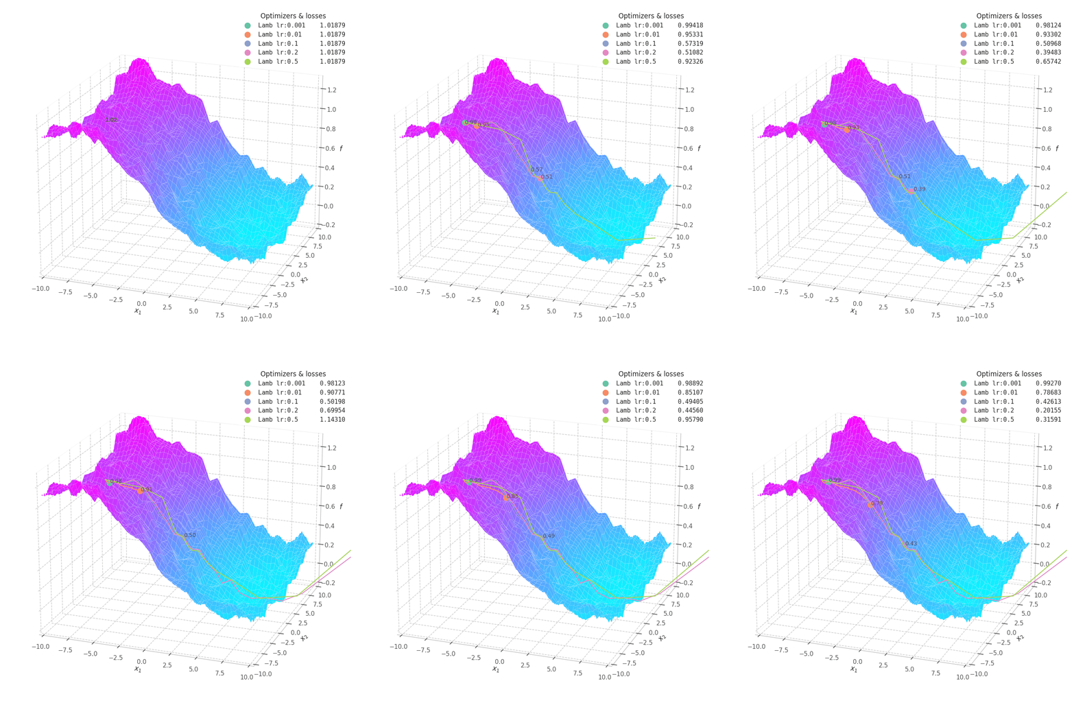
LAMB converges much faster than Adam. Notice that I dampened the learning rates (increasing lower ones and decreasing large ones) so the updates could still be visible in the animation.

The overshooting seen in Momentum-based methods is even more prominent here, as the updates are further scaled up by $\bm λ_t$ during initial steps when the parameters norms are usually high — though, granted, this phenomenon might be somewhat exaggerated here: it’s unlikely that real model parameters will assume absolute values as large as 10.

Naturally, LAMB decelerates when $\bm θ_t \to 0$, the point where $\bm λ_t$’s numerator is at its lowest. A decaying learning rate scheduling policy plays an important role in convergence for this method.

FTRL

FTRL is an optimization strategy that aims to achieve a good (effective) and sparse (regularized) solution. Its acronym stands for “Follow The (Proximally) Regularized Leader”, and it is first described by McMahan et al. [23]

FTRL’s update step is performed as follows.

where $\eta_t$ is the learning rate schedule originally set in the paper, inversely proportional to the training step ($\eta_t=\frac{1}{\sqrt{t}}$) and $\sigma_t$ is the $L_2$ coefficient s.t. $\sigma_{1:t}=\frac{1}{\eta_t}$. A hasten read of Eq. 12 may suggest to the reader the necessity of keeping track of all previous $\bm θ_s$. Fortunately, this equation can be rewritten [23] as:

FTRL employs both $L_1$ and $L_2$ regularization directly into the optimization objective function, modulated by hyperparameters $λ_1$ and $\sigma_s$, respectively; and it has been successfully employing when training large Natural Language Processing models, often trained over tasks represented by high-dimensional, sparsely represented feature spaces.

FTRL is implemented as follows in tensorflow/Keras:

where $\gamma$ is the learning rate reduction rate, commonly defined as $-0.5$.

def get_ftrl_with_different_lrs():
  return [
    ("FTRL lr: 0.001", tf.optimizers.Ftrl(learning_rate=0.001)),
    ("FTRL lr: 0.01", tf.optimizers.Ftrl(learning_rate=0.010)),
    ("FTRL lr: 0.1", tf.optimizers.Ftrl(learning_rate=0.100)),
    ("FTRL lr: 1.0", tf.optimizers.Ftrl(learning_rate=1.000)),
    ("FTRL lr:10.0", tf.optimizers.Ftrl(learning_rate=10.000)),
  ]

#@title $f_5$ - FTRL
opts = get_ftrl_with_different_lrs()
opt_points, opt_grads = optimize_all_w_opt(f5, opts, p0=[[9., 9.]])
f = f5(z[..., 0], z[..., 1], *positional_noise(z)).numpy()  # Loss at every grid-point.
y = {label: f5(points[..., 0], points[..., 1], *positional_noise(points)).numpy()
     for label, points in opt_points.items()}
fig, ax, handlers, L, ani = plot_surface_and_steps(
  opt_points, opt_grads, y, f, view=(40, -70), zlim=(.0, 1.5), legend=True)
ani.save("f5-ftrl-lr001-10.gif")

#@title $f_4$ - FTRL
opts = get_ftrl_with_different_lrs()
opt_points, opt_grads = optimize_all_w_opt(f4, opts, p0=[[-7.5, -1.0]])
f = f4(z[..., 0], z[..., 1], *positional_noise(z)).numpy()  # Loss at every grid-point.
y = {label: f4(points[..., 0], points[..., 1], *positional_noise(points)).numpy()
     for label, points in opt_points.items()}
fig, ax, handlers, L, ani = plot_surface_and_steps(
  opt_points, opt_grads, y, f, view=(20, -70), zlim=(-0.2, 1.3), legend=True)
ani.save("f4-ftrl-lr001-10.gif")

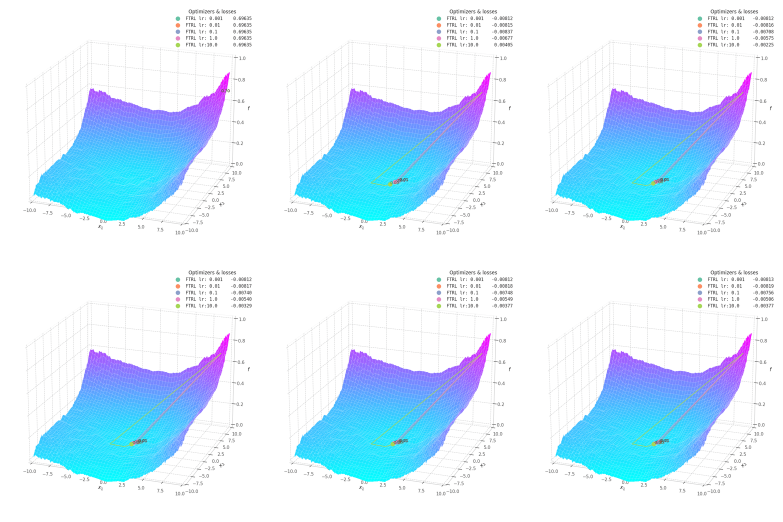
In my experiments, FTRL converged much faster than other algorithms, though it was particularly sensitive to noise, plateaus, and local minima. More specifically, most configurations resulted in a less-than-optimal solution for surface $f_4$, and no configuration was sufficient to transverse the local optimum plateau found in $f_1$ (which is easily optimized by Momentum, Adam and Lion).

Surface Transversing with Modern Optimizers

With a few tweaks, we can visualize how each and every of these optimization methods perform over the surface equations previously defined. Some of them are adaptive, and some are not. Thus, we are forced to use different hyper-parameters for each one of them. I picked the ones that shown good results in the previous sections, but doing some cross-validation over each surface might result in better behavior from some (or all) of the algorithms.

def get_optimizers(wd=None):
  return [
    ("SGD", tf.optimizers.SGD(learning_rate=10., weight_decay=wd)),
    ("NAG", tf.optimizers.SGD(learning_rate=10., momentum=0.9, nesterov=True, weight_decay=wd)),
    ("RMS", tf.optimizers.RMSprop(learning_rate=1., weight_decay=wd)),
    ("AdaGrad", tf.optimizers.Adagrad(learning_rate=10., weight_decay=wd)),
    ("Adam", tf.optimizers.AdamW(learning_rate=1., weight_decay=wd or 0.)),
    ("Adamax", tf.optimizers.Adamax(learning_rate=1., weight_decay=wd)),
    ("NAdam", tf.optimizers.Nadam(learning_rate=1., weight_decay=wd)),
    ("Lion", tf.optimizers.Lion(learning_rate=1., weight_decay=wd)),
    ("Lamb", tf.optimizers.Lamb(learning_rate=1., weight_decay=wd)),
    ("FTRL", tf.optimizers.Ftrl(learning_rate=1., weight_decay=wd)),
  ]

#@title $f_0$
_f = f0
p0 = [[9., 9.]]
opts = get_optimizers(wd=None)
opt_points, opt_grads = optimize_all_w_opt(_f, opts, p0=p0)
f = _f(z[..., 0], z[..., 1], *positional_noise(z)).numpy()  # Loss at every grid-point.
y = {label: _f(points[..., 0], points[..., 1], *positional_noise(points)).numpy() for label, points in opt_points.items()}
fig, ax, handlers, L, ani = plot_surface_and_steps(opt_points, opt_grads, y, f, view=(50, -70), zlim=(.0, 1.5), legend=False)
ani.save("suf_00.gif")

fig, ax, ani = plot_loss_in_time(y, zlim="auto")
ani.save("loss_00.gif")

#@title $f_1$
_f = f1
p0 = [[9., 9.]]
opts = get_optimizers(wd=None)
opt_points, opt_grads = optimize_all_w_opt(_f, opts, p0=p0)
f = _f(z[..., 0], z[..., 1], *positional_noise(z)).numpy()  # Loss at every grid-point.
y = {label: _f(points[..., 0], points[..., 1], *positional_noise(points)).numpy() for label, points in opt_points.items()}
fig, ax, handlers, L, ani = plot_surface_and_steps(opt_points, opt_grads, y, f, view=(20, -70), zlim=(.0, 1.0), legend=False)
ani.save("suf_01.gif")

fig, ax, ani = plot_loss_in_time(y, zlim="auto")
ani.save("loss_01.gif")

#@title $f_2$
_f = f2
p0 = [[7.5, -0.5]]
opts = get_optimizers(wd=None)
opt_points, opt_grads = optimize_all_w_opt(_f, opts, p0=p0)
f = _f(z[..., 0], z[..., 1], *positional_noise(z)).numpy()  # Loss at every grid-point.
y = {label: _f(points[..., 0], points[..., 1], *positional_noise(points)).numpy() for label, points in opt_points.items()}
fig, ax, handlers, L, ani = plot_surface_and_steps(opt_points, opt_grads, y, f, view=(30, -70), zlim=(-1.0, 1.0), legend=False)
ani.save("suf_02.gif")

fig, ax, ani = plot_loss_in_time(y, zlim="auto")
ani.save("loss_02.gif")

#@title $f_3$
_f = f3
p0 = [[-9.0, -2.5]]
opts = get_optimizers(wd=None)
opt_points, opt_grads = optimize_all_w_opt(_f, opts, p0=p0)
f = _f(z[..., 0], z[..., 1], *positional_noise(z)).numpy()  # Loss at every grid-point.
y = {label: _f(points[..., 0], points[..., 1], *positional_noise(points)).numpy() for label, points in opt_points.items()}
fig, ax, handlers, L, ani = plot_surface_and_steps(opt_points, opt_grads, y, f, view=(20, -70), zlim=(-1.4, 1.4), legend=False)
ani.save("suf_03.gif")

fig, ax, ani = plot_loss_in_time(y, zlim="auto")
ani.save("loss_03.gif")

#@title $f_4$
_f = f4
p0 = [[-7.5, -1.0]]
opts = get_optimizers(wd=None)
opt_points, opt_grads = optimize_all_w_opt(_f, opts, p0=p0)
f = _f(z[..., 0], z[..., 1], *positional_noise(z)).numpy()  # Loss at every grid-point.
y = {label: _f(points[..., 0], points[..., 1], *positional_noise(points)).numpy() for label, points in opt_points.items()}
fig, ax, handlers, L, ani = plot_surface_and_steps(opt_points, opt_grads, y, f, view=(20, -70), zlim=(-0.2, 1.3), legend=False)
ani.save("suf_04.gif")

fig, ax, ani = plot_loss_in_time(y, zlim="auto")
ani.save("loss_04.gif")

#@title $f_5$
_f = f5
p0 = [[9.0, 9.0]]
opts = get_optimizers(wd=None)
opt_points, opt_grads = optimize_all_w_opt(_f, opts, p0=p0)
f = _f(z[..., 0], z[..., 1], *positional_noise(z)).numpy()  # Loss at every grid-point.
y = {label: _f(points[..., 0], points[..., 1], *positional_noise(points)).numpy() for label, points in opt_points.items()}
fig, ax, handlers, L, ani = plot_surface_and_steps(opt_points, opt_grads, y, f, view=(20, -100), zlim=(-1.5, 1.3), legend=False)
ani.save("suf_05.gif")

fig, ax, ani = plot_loss_in_time(y, zlim="auto")
ani.save("loss_05.gif")

Previous Next

Final Considerations

In this post, I tried to bring a more intuitive visual representation for the optimization process conducted by the various optimization methods found in modern Machine Learning literature.

While we focused on 3-dimensional toy problems, techniques for visualization of the optimization landscape of higher order problems have become increasingly more popular nowadays. You can read more on this topic on the paper “Visualizing the Loss Landscape of Neural Nets” [2], which describes early strategies for representing high-order optimization landscapes. Today, visualization tools have evolved to even more complex strategies, many of which can be found at the losslandscape website.

Finally, while AdamW is the go-to optimizer used in literature (although SGD with momentum is often employed in Kaggle competitions), it is interesting to understand the motivation and objective behind each method. By detailing them and showing their application with visual examples, it is my hope that the reader can better understand their inner workings, as well as their assumptions, advantages, and shortcomings.

References

1. A. F. Agarap, “Deep learning using rectified linear units (relu),” arXiv preprint arXiv:1803.08375, 2018.
2. H. Li, Z. Xu, G. Taylor, C. Studer, and T. Goldstein, “Visualizing the loss landscape of neural nets,” Advances in neural information processing systems, vol. 31, 2018,Available at: https://arxiv.org/pdf/1712.09913
3. L. Bottou, “Stochastic gradient descent tricks,” in Neural Networks: Tricks of the Trade: Second Edition, Springer, 2012, pp. 421–436.
4. R. Bro and A. K. Smilde, “Principal Component Analysis,” Analytical methods, vol. 6, no. 9, pp. 2812–2831, 2014.
5. T.-W. Lee and T.-W. Lee, Independent component analysis. Springer, 1998.
6. J. Shlens, “A tutorial on independent component analysis,” arXiv preprint arXiv:1404.2986, 2014.
7. G. G. Thomas Lee and E. Henning, “Momentum,” SYSEN5800 Fall 2021. 2021.Available at: https://optimization.cbe.cornell.edu/index.php?title=Momentum
8. G. Goh, “Why Momentum Really Works,” Distill, 2017, doi: 10.23915/distill.00006.
9. Y. Nesterov, “A method for solving the convex programming problem with convergence rate O (1/k2),” in Dokl akad nauk Sssr, 1983, vol. 269, p. 543.
10. T. Dozat, “Incorporating Nesterov Momentum into Adam,” 2016,Available at: https://cs229.stanford.edu/proj2015/054_report.pdf
11. G. Hinton, N. Srivastava, and K. Swersky, “Neural Networks for Machine Learning: Lecture 6a - Overview of mini-‐batch gradient descent.” Lecture notes.Available at: http://www.cs.toronto.edu/t̃ijmen/csc321/slides/lecture_slides_lec6.pdf
12. J. Duchi, E. Hazan, and Y. Singer, “Adaptive subgradient methods for online learning and stochastic optimization.,” Journal of machine learning research, vol. 12, no. 7, 2011.
13. D. Villarraga, “AdaGrad,” Cornell University Computational Optimization Open Textbook. 2021.Available at: https://optimization.cbe.cornell.edu/index.php?title=AdaGrad
14. D. P. Kingma, “Adam: A method for stochastic optimization,” arXiv preprint arXiv:1412.6980, 2014.
15. I. Goodfellow, Y. Bengio, and A. Courville, Deep Learning. MIT Press, 2016.
16. T. Dozat, “Incorporating nesterov momentum into adam,” 2016.
17. X. Chen et al., “Symbolic discovery of optimization algorithms,” Advances in neural information processing systems, vol. 36, 2024.
18. A. Krizhevsky, “One weird trick for parallelizing convolutional neural networks,” arXiv preprint arXiv:1404.5997, 2014.
19. Y. You, I. Gitman, and B. Ginsburg, “Scaling SGD Batch Size to 32K for ImageNet Training,” arXiv preprint arXiv:1708.03888, vol. 6, no. 12, p. 6, 2017.
20. Y. You et al., “Large batch optimization for deep learning: Training bert in 76 minutes,” arXiv preprint arXiv:1904.00962, 2019.
21. G. Garrigos and R. M. Gower, “Handbook of convergence theorems for (stochastic) gradient methods,” arXiv preprint arXiv:2301.11235, 2023.
22. S. Ghadimi and G. Lan, “Stochastic first-and zeroth-order methods for nonconvex stochastic programming,” SIAM journal on optimization, vol. 23, no. 4, pp. 2341–2368, 2013.
23. H. B. McMahan et al., “Ad click prediction: a view from the trenches,” in Proceedings of the 19th ACM SIGKDD international conference on Knowledge discovery and data mining, 2013, pp. 1222–1230.