
This post is based on an assignment submitted to a Machine Learning class at Universidade Estadual de Campinas, and its challenges were equally divided among Jonathan and I.
Here, our goal is to apply unsupervised learning methods to solve clustering and dimensionality reduction in two distinct task. We implemented the K-Means and Hierarchical Clustering algorithms (and their evaluation metrics) from the ground up. Results are presented over three distinct datasets, including a bonus color quantization example.
import numpy as np
import TensorFlow as tf
import seaborn as sns
import logging
from math import ceil
from typing import Dict, List, Set, Any, Union, Callable

import pandas as pd
import TensorFlow_datasets as tfds
import matplotlib.pyplot as plt
from sklearn.model_selection import ParameterGrid
from sklearn.decomposition import PCA


class Config:
  class cluster_dat:
    k_init_method = 'kpp'
    k_max = 10
    repeats = 100
    steps = 30
    tol = .0001

    test_size = 0.1
    source = '/content/drive/MyDrive/datasets/MO444/cluster.dat'

  class cali:
    k_init_method = 'kpp'
    k_max = 10
    repeats = 100
    steps = 100
    tol = .0001

    sample_size = 500
    test_size = 0.1

  class tf_flowers:
    colors = 128  # k, actually
    training_samples = 10000
    steps = 100
    tol = .01

    test_size = 0.1
    batch_size = 8
    buffer_size = batch_size * 8
    image_sizes = (150, 150)
    channels = 3
    shape = (*image_sizes, channels)

  class run:
    palette = sns.color_palette("husl", 3)
    # seed = 472
    seed = 821


tf.random.set_seed(Config.run.seed)
np.random.seed((Config.run.seed//4 + 41) * 3)

sns.set(style="whitegrid")
sns.set_palette(Config.run.palette)


def split_dataset(*tensors, test_size):
  s = tensors[0].shape[0]

  indices = tf.range(s)
  indices = tf.random.shuffle(indices)

  train_indices, test_indices = (indices[int(test_size*s):],
                                 indices[:int(test_size*s)])

  return sum(((tf.gather(x, train_indices, axis=0),
               tf.gather(x, test_indices, axis=0))
              for x in tensors), ())

def standardize(x, center=True, scale=True, return_stats=False, axis=0):
  """Standardize data based on its mean and standard-deviation.
  """
  u, s = None, None
  if center:
    u = tf.reduce_mean(x, axis=axis, keepdims=True)
    x = x-u

  if scale:
    s = tf.math.reduce_std(x, axis=axis, keepdims=True)
    x = tf.math.divide_no_nan(x, s)

  if return_stats:
    return x, (u, s)

  return x

def inverse_standardize(x, u, s):
  if s is not None: x = x*s
  if u is not None: x = x+u
  return x

def size_in_mb(x):
  return tf.reduce_prod(x.shape)*8 / 1024**2

def visualize_clusters(*sets, title=None, full=True, legend=True, figsize=(9, 6)):
  d = pd.concat([
    pd.DataFrame({
      'x': features[:, 0],
      'y': features[:, 1],
      'cluster': [f'cluster {l}' for l in np.asarray(labels).astype(str)],
      'subset': [subset] * features.shape[0]
    })
    for features, labels, subset, _ in sets
  ])

  if full: plt.figure(figsize=figsize)
  if title: plt.title(title)

  markers = {s: m for _, _, s, m in sets}
  sns.scatterplot(data=d, x='x', y='y', hue='cluster', style='subset', markers=markers, legend=legend)
  if full: plt.tight_layout()

def visualize_images(
    image,
    title=None,
    rows=2,
    cols=None,
    cmap=None,
    figsize=(14, 6)
):
  if image is not None:
    if isinstance(image, list) or len(image.shape) > 3:  # many images
      plt.figure(figsize=figsize)
      cols = cols or ceil(len(image) / rows)
      for ix in range(len(image)):
        plt.subplot(rows, cols, ix+1)
        visualize_images(
          image[ix],
          cmap=cmap,
          title=title[ix] if title is not None and len(title) > ix else None)
      plt.tight_layout()
      return

    if isinstance(image, tf.Tensor): image = image.numpy()
    if image.shape[-1] == 1: image = image[..., 0]
    plt.imshow(image, cmap=cmap)

  if title is not None: plt.title(title)
  plt.axis('off')
Datasets
In this section, we present the datasets used in this assignment. They were selected considering their diverse nature, in order to visualize the behavior of clustering/dimensionality reduction techniques in different scenarios.
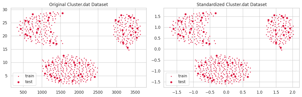
cluster.dat
This dataset was provided during class. It comprises 573 samples and 2 numeric features.
cluster_train = tf.constant(np.genfromtxt(Config.cluster_dat.source), tf.float32)

cluster_train, cluster_test = split_dataset(
  cluster_train,
  test_size=Config.cluster_dat.test_size
)

cluster_s_train, (c_u, c_s) = standardize(cluster_train, return_stats=True)
cluster_s_test = standardize(cluster_test)
plt.figure(figsize=(12, 4))
plt.subplot(121)
plt.title('Original Cluster.dat Dataset')
sns.scatterplot(x=cluster_train[:, 0], y=cluster_train[:, 1], label='train', marker='.', color='crimson')
sns.scatterplot(x=cluster_test[:, 0], y=cluster_test[:, 1], label='test', color='crimson');

plt.subplot(122)
plt.title('Standardized Cluster.dat Dataset')
sns.scatterplot(x=cluster_s_train[:, 0], y=cluster_s_train[:, 1], label='train', marker='.', color='crimson')
sns.scatterplot(x=cluster_s_test[:, 0], y=cluster_s_test[:, 1], label='test', color='crimson')

plt.tight_layout();
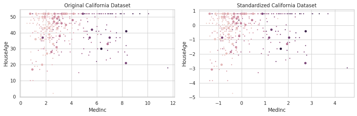
California
The california housing dataset was constructed by collecting information over all block groups from the 1990 Census. It comprises 20,640 samples and 9 features, associating the aforementioned blocks to the log of the median house value within them. Finally, blocks on average contain 1425.5 individuals [1].
Features are:
- MedInc: median income in block group;
- HouseAge: median house age in block group;
- AveRooms: average number of rooms per household;
- AveBedrms: average number of bedrooms per household;
- Population: block group population;
- AveOccup: average number of household members;
- Latitude: block group latitude;
- Longitude: block group longitude.
from sklearn.datasets import fetch_california_housing

cali = fetch_california_housing()
cali_feature_names = cali.feature_names

cali_x_train = cali.data.astype(np.float32)[:Config.cali.sample_size]
cali_y_train = cali.target.astype(np.float32)[:Config.cali.sample_size]

(cali_x_train, cali_x_test, cali_y_train, cali_y_test) = split_dataset(
  cali_x_train,
  cali_y_train,
  test_size=Config.cali.test_size,
)

cali_s_train, (b_u, b_s) = standardize(cali_x_train, return_stats=True)
cali_s_test = standardize(cali_x_test, us=(b_u, b_s))
plt.figure(figsize=(12, 4))
plt.subplot(121)
plt.title('Original California Dataset')
sns.scatterplot(x=cali_x_train[:, 0], y=cali_x_train[:, 1], hue=cali_y_train, marker='.', label='train', legend=False)
sns.scatterplot(x=cali_x_test[:, 0], y=cali_x_test[:, 1], hue=cali_y_test, label='test', legend=False)
plt.xlabel(cali_feature_names[0])
plt.ylabel(cali_feature_names[1])

plt.subplot(122)
plt.title('Standardized California Dataset')
sns.scatterplot(x=cali_s_train[:, 0], y=cali_s_train[:, 1], hue=cali_y_train, marker='.', label='train', legend=False)
sns.scatterplot(x=cali_s_test[:, 0], y=cali_s_test[:, 1], hue=cali_y_test, label='test', legend=False)
plt.xlabel(cali_feature_names[0])
plt.ylabel(cali_feature_names[1])
plt.tight_layout()

cali_x_train, cali_x_test = cali_s_train, cali_s_test
del cali_s_train, cali_s_test
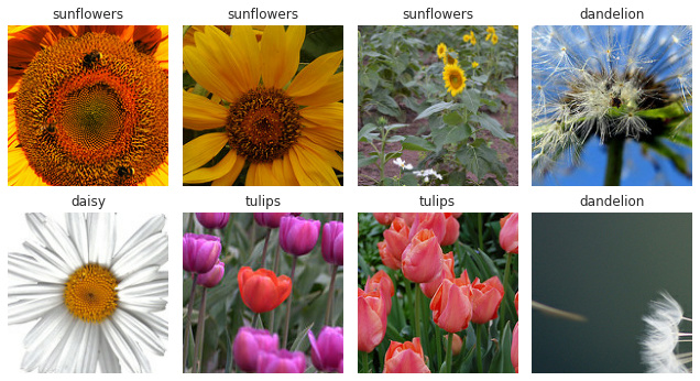
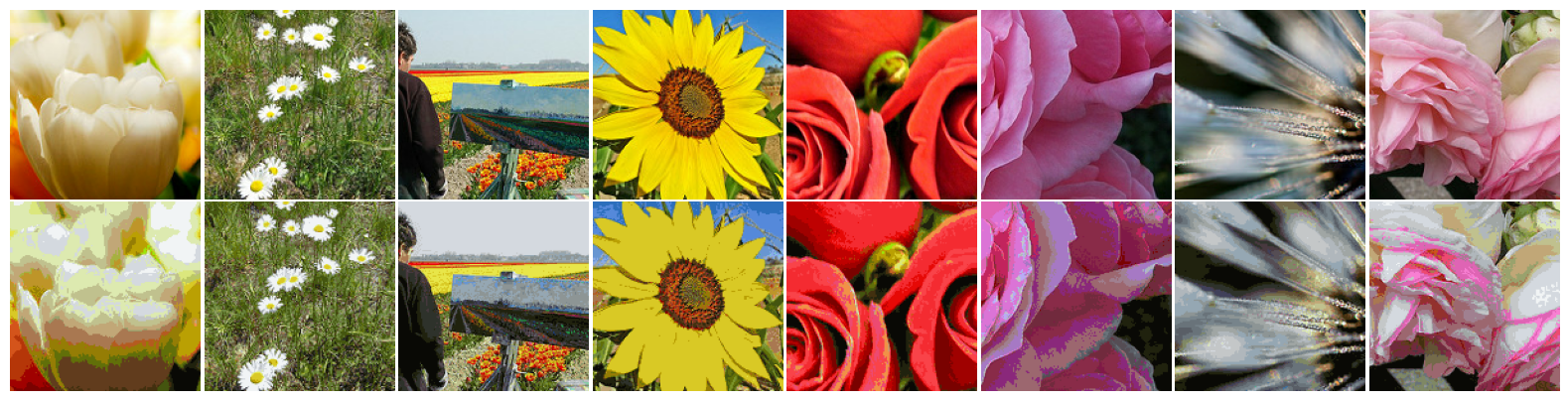
TF-Flowers
We utilize TF-Flowers dataset to illustrate the application of K-Means in Color Quantization. This dataset represents a multi-class (mono-label) image classification problem, and comprises 3,670 photographs of flowers associated with one of the following labels: dandelion, daisy, tulips, sunflowers or roses.
def preprocessing_fn(image, label):
  current = tf.cast(tf.shape(image)[:2], tf.float32)
  target = tf.convert_to_tensor(Config.tf_flowers.image_sizes, tf.float32)
  ratio = tf.reduce_max(tf.math.ceil(target / current))
  new_sizes = tf.cast(current*ratio, tf.int32)

  image = tf.image.resize(image, new_sizes, preserve_aspect_ratio=True)
  image = tf.image.resize_with_crop_or_pad(image, *Config.tf_flowers.image_sizes)

  return image, label

def prepare(ds):
  return (ds.shuffle(Config.tf_flowers.buffer_size)
            .map(preprocessing_fn, num_parallel_calls=tf.data.AUTOTUNE)
            .batch(Config.tf_flowers.batch_size, drop_remainder=True)
            .prefetch(tf.data.AUTOTUNE))

def load_tf_flowers():
  (train_ds, test_ds), info = tfds.load(
    'tf_flowers',
    split=['train[:50%]', 'train[50%:]'],
    with_info=True,
    as_supervised=True,
    shuffle_files=False)

  train_ds = prepare(train_ds)
  test_ds = prepare(test_ds)

  train_ds.info = info
  train_ds.int2str = info.features['label'].int2str

  return train_ds, test_ds

flowers_train_set, flowers_test_set = load_tf_flowers()

images, target = next(iter(flowers_train_set))
labels = [flowers_train_set.int2str(l) for l in target]
visualize_images(
  tf.cast(images, tf.uint8),
  labels,
  figsize=(9, 5)
)
Part-1: Clustering Methods
K-Means
Our K-Means implementation was developed on top of the TensorFlow library, and was expressed in its primal optimization form [2].
Let:
- $X$ be the set of observations
- $k\in\mathbb{Z}$ the number of clusters
- $C = \{C_1, C_2, \ldots, C_k\}$ a set of $k$ clusters, represented by their respective “centers” $\{c_1, c_2, \ldots, c_k\}$
A given sample $x\in X$ is said contained in cluster $C_i\in C$ $\iff i=\text{argmin}_j ||x-c_j||^2$. That is, $x$ is closer to $c_i$ than to any other $c_j, \forall j\in [1, k] \setminus \{i\}$.
K-Means’s prime form can be described as a non-linear optimization problem over the cost function $J(X, C)$:
\[\text{argmin}_C \sum_{i}^k \sum_{x\in C_i} \|x-c_i\|^2\]As this error is minimum when $c_i = \mu_i = \frac{1}{|C_i|}\sum_{x\in C_i} x$, we know the negative gradient $-\nabla J$ points out in the direction towards the centroids of the clusters in $C$, and this function can be optimized using Gradient Descent:
\[C^n := C^{n-1} - \lambda\nabla J\]Where $\lambda$ is the associated learning rate.
Algorithm
def kmeans_fit(
    x: tf.Tensor,
    c: tf.Variable,
    steps: int = 10,
    lr: float = .001,
    tol: float = 0.0001,
    verbose: int = 1,
    report_every: int = 10,
) -> tf.Tensor:
  """Learn the set of clusters that minimize the WSS loss function.

  Arguments
  ---------
  x: tf.Tensor (samples, features)
    samples from the dataset that we are studying
  c: tf.Variable (clusters, features)
    an initial set of clusters, used as starting point for the optimization process
  steps: int
    the number of optimization iterations
  lr: float
    the learning rate used to amortize the gradients
    in case batches of data are being passed
  tol: float
    minimum absolute loss variance between two consecutive
    iterations so converge is declared

  Returns
  -------
  tf.Tensor
    The list of clusters, a tensor of shape (clusters, features).
  """
  lr = tf.convert_to_tensor(lr, name='learning_rate')

  if verbose > 0:
    kmeans_report_evaluation('Step 0', x, c)

  p_loss = -1

  for step in range(1, steps+1):
    loss = kmeans_train_step(x, c, lr).numpy().item()

    if verbose > 1 and step % report_every == 0:
      kmeans_report_evaluation(f'Step {step}', x, c)

    diff_loss = abs(loss - p_loss)
    if diff_loss < tol:
      if verbose: print(f'\nEarly stopping as loss diff less than tol [{diff_loss:.4f} > {tol:.4f}]')
      break

    p_loss = loss

  if verbose == 1 or verbose > 1 and step % report_every:
    # last step, if not reported yet
    kmeans_report_evaluation(f'Step {step}', x, c)

  return c

def kmeans_train_step(
    x: tf.Tensor,
    c: tf.Variable,
    lr: float,
) -> tf.Variable:
  with tf.GradientTape() as t:
    loss = KMeansMetrics.WCSS(x, c)

  dldc = t.gradient(loss, c)
  c.assign_sub(lr * dldc)

  return tf.reduce_sum(loss)

def kmeans_test_step(
    x: tf.Tensor,
    c: tf.Tensor
) -> Dict[str, float]:
  k, f = c.shape

  d = k_distance(x, c)
  y = tf.argmin(d, axis=-1)

  s = KMeansMetrics.samples_per_cluster(x, c)
  wss_ = KMeansMetrics.WCSS(x, c)
  bss_ = KMeansMetrics.BCSS(x, c)
  sil_ = KMeansMetrics.silhouette(x, y, k)
  wc_sil_ = KMeansMetrics.wc_avg_silhouette(sil_, y, k)

  return dict(zip(
    ('Loss', 'WCSS', 'BCSS', 'Silhouette', 'WC Silhouette', 'Samples'),
    (tf.reduce_sum(wss_).numpy(),
    tf.reduce_mean(wss_).numpy(),
    tf.reduce_mean(bss_).numpy(),
    tf.reduce_mean(sil_).numpy(),
    tf.reduce_mean(wc_sil_).numpy(),
    tf.cast(s, tf.int32).numpy())
  ))

def kmeans_report_evaluation(tag, x, c):
  report = kmeans_test_step(x, c)

  print(tag)
  lpad = max(map(len, report)) + 2
  rpad = 12

  for metric, value in report.items():
    print(f'  {metric}'.ljust(lpad), '=', str(value.round(4)).rjust(rpad))
def kmeans_search(
  x: tf.Tensor,
  k_max: int,
  init: str = 'kpp',
  steps: int = 10,
  lr: float = .001,
  tol: float = 0.0001,
  repeats: int = 10,
  verbose: int = 1
) -> pd.DataFrame:
  """N-Repeated Line-Search for K Parameter Optimization.

  Arguments
  ---------
  x: tf.Tensor (samples, features)
    samples from the dataset that we are studying
  k_max: int
    maximum number of clusters used when searching
  init: str
    initialization method used.
    Options are:
      - normal: normally distributed clusters, following the training set's distribution.
      - uniform: uniformally distributed clusters, following the training set's distribution.
      - random_points: draw points from the training set and use them as clusters.
      - kpp: k-means++ algorithm

  steps: int
    the number of optimization iterations
  lr: float
    the learning rate used to amortize the gradients
    in case batches of data are being passed
  tol: float
    minimum absolute loss variance between two consecutive
    iterations so converge is declared

  Returns
  -------
    pd.DataFrame
      The search results report.
  """
  results = []

  init = get_k_init_fn_by_name(init)

  for k in range(2, k_max + 1):
    if verbose > 0: print(f'k: {k}, performing {repeats} tests')

    for r in range(repeats):
      clusters = tf.Variable(init(x, k), name=f'ck{k}')
      clusters = kmeans_fit(x, clusters, steps=steps, lr=lr, tol=tol, verbose=0)
      metrics = kmeans_test_step(x, clusters)

      results += [{'k': k, 'repetition': r, **metrics}]

      if verbose > 1: print('.', end='' if r < repeats-1 else '\n')

  return pd.DataFrame(results)
def kmeans_predict(
    x: tf.Tensor,
    c: tf.Tensor
) -> tf.Tensor:
  """Predict cluster matching for dataset {x} based on pre-trained clusters {c}.
  """
  d = k_distance(x, c)
  d = tf.argmin(d, -1, tf.int32)

  return d
Evaluation Metrics
In this section, we describe the metrics employed to evaluate K-Means, as well as their actual python implementations.
-
Within Cluster Sum of Squares (WCSS)
Computes the sum (macro average, really) of distances between each sample and its respective cluster’s centroid [3]. This function (K-Means primal form) is used as loss function in our opt function.
Def: $Σ_i^k Σ_{x \in c_i} ||x - \bar{x}_{c_i}||^2$
-
Between Cluster Sum of Squares (BCSS)
Computes the sum (macro average, really) distance between each sample $x\in c_i$ to the centroids of the clusters $c_k\in C\setminus c_i$ [3].
Def: $Σ_i^k Σ_{x \in X \setminus c_i} ||x - \bar{x}_{c_i}||^2$
-
Silhouette [4]
In our silhouette implementation, we used the one-hot encoding representation to select the corresponding samples of each cluster when computing avg. inter/intra cluster distance between samples $\{x_0, x_1, \ldots, x_n\}$ and clusters $\{c_0, c_1,\ldots, l_k\}$:
\[\begin{align} D &= \begin{bmatrix} d_{00} & d_{01} & d_{02} & \ldots & d_{0n} \\ d_{10} & d_{11} & d_{12} & \ldots & d_{1n} \\ \ldots \\ d_{n0} & d_{n1} & d_{n2} & \ldots & d_{nn} \\ \end{bmatrix} \\ y &= \begin{bmatrix} 0 & 1 & 2 & 0 & 1 & 2 & \ldots \end{bmatrix} \\ D \cdot \text{onehot}(y) &= \begin{bmatrix} \sum_i d_{0,i}[y_i=0] & \sum_i d_{0,i}[y_i=1] & \ldots & \sum_i d_{0,i}[y_i=k]\\ \sum_i d_{1,i}[y_i=0] & \sum_i d_{1,i}[y_i=1] & \ldots & \sum_i d_{1,i}[y_i=k]\\ \ldots\\ \sum_i d_{n,i}[y_i=0] & \sum_i d_{n,i}[y_i=1] & \ldots & \sum_i d_{n,i}[y_i=k]\\ \end{bmatrix} \end{align}\]
def k_distance(x, c):
  """Calculate the squared distance from each
    point in {x} to each point in {c}.
  """
  s, f = x.shape
  k, _ = c.shape

  x = x[:, tf.newaxis, ...]
  c = c[tf.newaxis, ...]

  d = tf.reduce_sum((x - c)**2, axis=-1)

  return d

class KMeansMetrics:
  @staticmethod
  def WCSS(x, c):
    """Within Cluster Sum of Squares.

    Note:
      This function returns a vector with the distances between points and their
      respective clusters --- without adding them ---, as `tf.GradientTape#gradients`
      will automatically add these factors together to form the gradient.

      We choose this formulation so this same code can be conveniently averaged (instead of summed)
      during evaluation, and behave consistently between sets with different cardinality (e.g. train, test).

    """
    d = k_distance(x, c)
    d = tf.reduce_min(d, axis=-1)

    return d

  @staticmethod
  def BCSS(x, c):
    """Between Cluster Sum of Squares.
    """
    d = k_distance(x, c)
    di = tf.reduce_min(d, axis=-1)
    db = tf.reduce_sum(d, axis=-1) - di

    return db

  @staticmethod
  def silhouette(x, y, k):
    """Silhouette score as defined by Scikit-learn.
    """
    d = k_distance(x, x)
    h = tf.one_hot(y, k)
    du = tf.math.divide_no_nan(
      d @ h,
      tf.reduce_sum(h, axis=0)
    )

    a = du[h == 1]
    b = tf.reshape(du[h != 1], (-1, k-1))  # (k-1), as one of these distances was selected into `a`.
    b = tf.reduce_min(b, axis=-1)          # using `tf.reduce_min` as sklearn defines Silhouette's
                                           # `b` as "nearest-cluster distance" [2].
    return tf.math.divide_no_nan(
      b - a,
      tf.maximum(a, b)
    )

  @staticmethod
  def samples_per_cluster(x, c):
    C_i = k_distance(x, c)
    C_i = tf.argmin(C_i, axis=-1)
    C_i = tf.cast(C_i, tf.int32)
    C_i = tf.math.bincount(C_i, minlength=c.shape[0])
    C_i = tf.cast(C_i, tf.float32)

    return C_i

  @staticmethod
  def wc_avg_silhouette(s, y, k):
    s = tf.reshape(s, (-1, 1))
    h = tf.one_hot(y, k)
    sc = tf.reduce_mean(s * h, axis=0)

    return sc
Clusters Initialization
def normal_clusters(x, k):
  """Normal clusters.

  Draw random clusters that follow the same distribution as the training set `x`.

  """
  f = x.shape[-1]

  u, st = (tf.math.reduce_mean(x, axis=0),
           tf.math.reduce_std(x, axis=0))

  return tf.random.normal([k, f]) * st + u


def uniform_clusters(x, k):
  """Uniform clusters.

  Draw uniformly random clusters that are strictly contained within the min and max
  values present in the training set `x`. Useful when drawing image pixels (see
  Application over The TF-Flowers Dataset section for usage).

  """
  f = x.shape[-1]

  return tf.random.uniform((k, f), tf.reduce_min(x), tf.reduce_max(x))


def random_points_clusters(x, k):
  """Random Points clusters.

  Draw clusters that coincide with the points in the training set `x`.

  """
  samples = x.shape[0]
  indices = tf.random.uniform([k], minval=0, maxval=samples, dtype=tf.dtypes.int32)

  return tf.gather(x, indices, axis=0)


def kpp_clusters(x, k, device='CPU:0'):
  """K-Means++ clusters.

  Draw clusters using the k-means++ procedure.

  Note: this section relies heavely on numpy, as we were unable to implement the
  function `np.random.choice(..., p=[0.1, 0.2, ...])` in TensorFlow. We therefore
  force the code execution of this section in the CPU.
  You can override this behavior by passing `device='GPU:0'` as a function argument.

  """
  s, f = x.shape

  with tf.device(device):
    c = np.random.choice(s, size=[1])
    d = k_distance(x, x)

    for i in range(1, k):
      d_xc = tf.gather(d, c, axis=1)
      d_xc = tf.reduce_min(d_xc, axis=1)
      pr = tf.math.divide_no_nan(
        d_xc,
        tf.reduce_sum(d_xc)
      )
      ci = np.random.choice(s, size=[1], p=pr.numpy())
      c = tf.concat((c, ci), axis=0)

  return tf.gather(x, c, axis=0)


def get_k_init_fn_by_name(name):
  return globals()[f'{name}_clusters']
initializations = (normal_clusters,
                   uniform_clusters,
                   random_points_clusters,
                   kpp_clusters)

plt.figure(figsize=(16, 4))

for ix, ini in enumerate(initializations):
  c = ini(cluster_train, 3)
  p_tr = kmeans_predict(cluster_train, c)
  p_te = kmeans_predict(cluster_test, c)

  plt.subplot(1, len(initializations), ix+1)
  visualize_clusters(
    (cluster_train, p_tr, 'train', '.'),
    (cluster_test, p_te, 'test', 'o'),
    (c, [0, 1, 2], 'clusters', 's'),  # labels for clusters are trivial (0, 1, 2, ...)
    title=ini.__name__,
    legend=False,
    full=False
  )

plt.tight_layout();
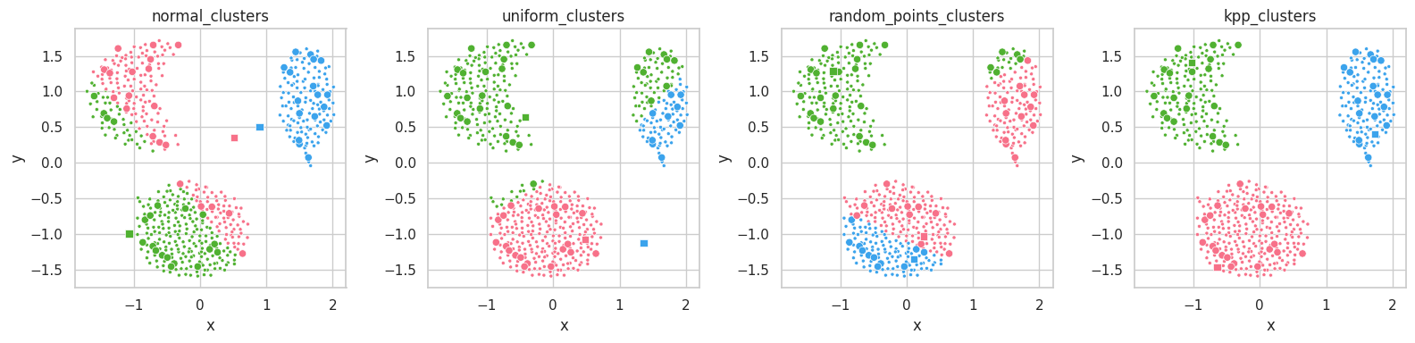
random_points_clusters) produces better results than uniform or normal clusters, while kpp_clusters results in an almost perfect clustering from the start.
The normal_clusters initialization procedure considers the mean and standard deviation of the training set’s distribution, which means points drawn from this procedure will belong to the set’s distribution and assume reasonable values in each feature.
For datasets with complex shapes (with holes close to its features’ average values), this method might create unreasonable clusters, which lie on empty sections of the dimensional space. In the example above, we see clusters lying in between the data masses.
The uniform initialization behaves similarly to random_clusters, but it is ensured to always draw samples with feature values within their respective valid intervals.
On the other hand, random_points_clusters draws points from the training set itself, which will invariantly assume valid values in each feature, being valid cluster’s centroid candidates. Its drawback lies on the uniform selection procedure itself: sampling datasets containing unbalanced masses will likely result in clusters being drawn from a same mass.
Finally, K-Means++ [5] seems to already separate the data masses correctly from the start. K-Means will mearly move these points to their respective data masses’ centroids.
ctr = cluster_train * c_s + c_u
cte = cluster_test * c_s + c_u

c0 = kpp_clusters(ctr, 3)
c1 = kpp_clusters(cluster_train, 3)

p0_train = kmeans_predict(ctr, c0)
p0_test = kmeans_predict(cte, c0)

p1_train = kmeans_predict(cluster_train, c1)
p1_test = kmeans_predict(cluster_test, c1)
plt.figure(figsize=(12, 4))
plt.subplot(121)
visualize_clusters(
  (ctr, p0_train, 'train', '.'),
  (cte, p0_test, 'test', 'o'),
  (c0, [0, 1, 2], 'clusters', 's'),         # labels for clusters are trivial (0, 1, 2, ...)
  title='Original Data Initial Clustering',
  full=False,
  legend=False
)

plt.subplot(122)
visualize_clusters(
  (cluster_train, p1_train, 'train', '.'),
  (cluster_test, p1_test, 'test', 'o'),
  (c1, [0, 1, 2], 'clusters', 's'),         # labels for clusters are trivial (0, 1, 2, ...)
  title='Standardized Data Initial Clustering',
  full=False,
  legend=False
)
plt.tight_layout();

del ctr, cte, c0, c1, p0_train, p0_test, p1_train, p1_test
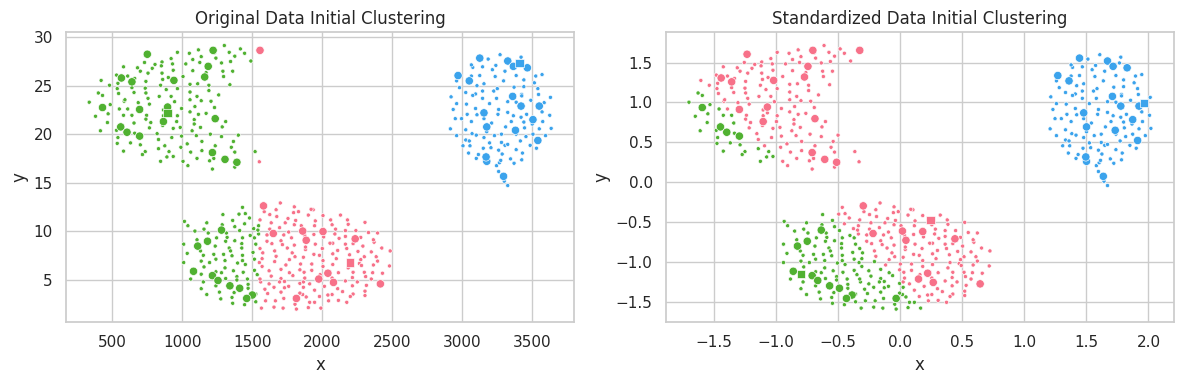
In the example above, the unstandardized feature $y$ ranged within the interval $[0, 30]$, which profoundly affected the $l^2$ distance. Conversely, variations in feature $x\in [250, 3750]$ caused a smaller impact on clustering configuration. In the second scatterplot, we notice all features belonging to the same interval, and contributing similarly to the distance function $l^2$.
Application over The Cluster.dat Dataset
An interesting application of clustering is image compression through color quantization. In this procedure, the RGB pixels in an image are clustered into $k$ groups, comprising the color book. The image can then be “compressed” by replacing each pixel by its cluster’s centroid’s identifier, which effectively reduces three floating point numbers to a single unsigned integer (plus the memory necessary to store the color book).
Searching K
%%time

report = kmeans_search(
  cluster_train,
  k_max=Config.cluster_dat.k_max,
  init=Config.cluster_dat.k_init_method,
  repeats=Config.cluster_dat.repeats,
  steps=Config.cluster_dat.steps,
  verbose=2
)
k: 2, performing 100 tests
....................................................................................................
k: 3, performing 100 tests
....................................................................................................
k: 4, performing 100 tests
....................................................................................................
k: 5, performing 100 tests
....................................................................................................
k: 6, performing 100 tests
....................................................................................................
k: 7, performing 100 tests
....................................................................................................
k: 8, performing 100 tests
....................................................................................................
k: 9, performing 100 tests
....................................................................................................
k: 10, performing 100 tests
....................................................................................................
CPU times: user 4min, sys: 1.32 s, total: 4min 2s
Wall time: 3min 53s
report.groupby('k').mean().round(2)
| k | repetition | Loss | WCSS | BCSS | Silhouette | WC Silhouette | Samples |
|---|---|---|---|---|---|---|---|
| 2 | 49.5 | 576.63 | 1.12 | 5.81 | 0.63 | 0.32 | [295.93, 220.07] |
| 3 | 49.5 | 139.47 | 0.27 | 11.89 | 0.88 | 0.29 | [176.21, 166.32, 173.47] |
| 4 | 49.5 | 110.74 | 0.21 | 15.67 | 0.72 | 0.18 | [143.63, 137.19, 127.55, 107.63] |
| 5 | 49.5 | 92.67 | 0.18 | 19.90 | 0.66 | 0.13 | [115.62, 108.89, 113.64, 95.02, 82.83] |
| 6 | 49.5 | 78.08 | 0.15 | 23.91 | 0.62 | 0.10 | [96.23, 96.44, 86.15, 86.56, 76.25, 74.37] |
| 7 | 49.5 | 66.92 | 0.13 | 27.78 | 0.59 | 0.08 | [80.53, 80.69, 83.48, 72.83, 69.0, 65.91, 63.56] |
| 8 | 49.5 | 57.72 | 0.11 | 31.94 | 0.58 | 0.07 | [74.07, 71.94, 71.97, 63.15, 63.07, 59.2, 57.1... |
| 9 | 49.5 | 51.29 | 0.10 | 35.79 | 0.56 | 0.06 | [66.08, 65.78, 59.17, 56.12, 57.82, 55.57, 52.... |
| 10 | 49.5 | 45.16 | 0.09 | 40.29 | 0.54 | 0.05 | [55.91, 55.6, 56.11, 54.11, 52.36, 51.56, 48.5... |
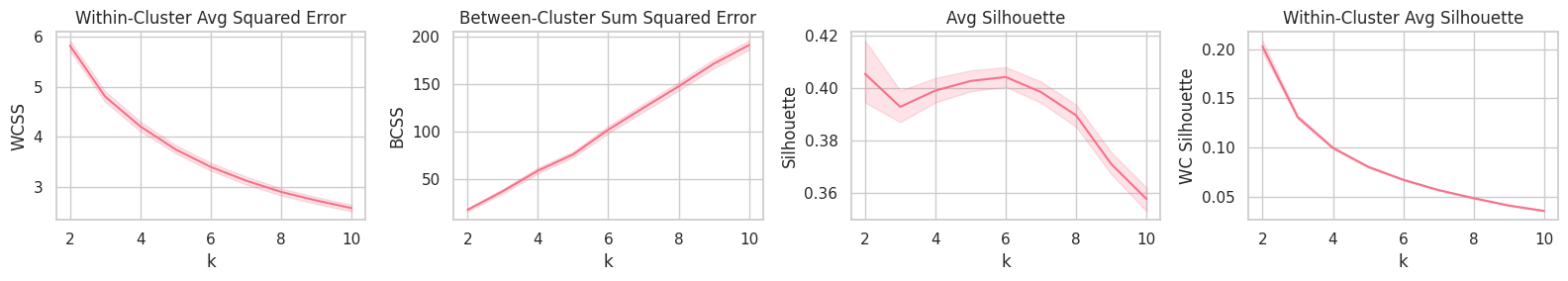
plt.figure(figsize=(16, 3))
plt.subplot(141).set_title('Within-Cluster Avg Squared Error'); sns.lineplot(data=report, x='k', y='WCSS')
plt.subplot(142).set_title('Between-Cluster Sum Squared Error'); sns.lineplot(data=report, x='k', y='BCSS')
plt.subplot(143).set_title('Avg Silhouette'); sns.lineplot(data=report, x='k', y='Silhouette')
plt.subplot(144).set_title('Within-Cluster Avg Silhouette'); sns.lineplot(data=report, x='k', y='WC Silhouette')
plt.tight_layout();
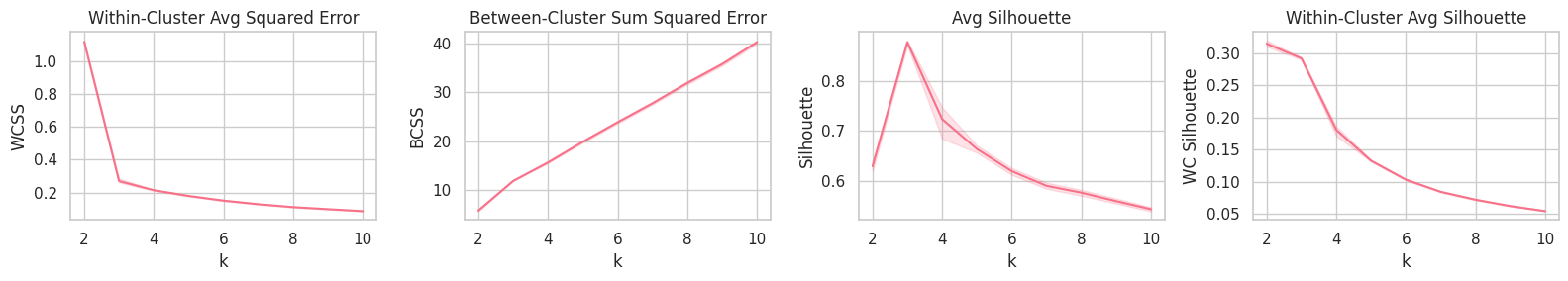
Training
best_k = report.groupby('k').mean().Silhouette.idxmax()

print(f'Best K (highest Silhouette) found: {best_k}')
Best K (highest Silhouette) found: 3
clusters = tf.Variable(normal_clusters(cluster_train, best_k), name=f'ck{best_k}')
clusters = kmeans_fit(
  cluster_train,
  clusters,
  steps=Config.cluster_dat.steps,
  tol=Config.cluster_dat.tol,
  verbose=2
)
Step 0
  Loss          =     766.6576
  WCSS          =       1.4858
  BCSS          =       8.0952
  Silhouette    =       0.4539
  WC Silhouette =       0.1513
  Samples       = [225 178 113]
Step 10
  Loss          =     136.2397
  WCSS          =        0.264
  BCSS          =      11.5245
  Silhouette    =       0.8801
  WC Silhouette =       0.2934
  Samples       = [252 151 113]
Step 20
  Loss          =      135.358
  WCSS          =       0.2623
  BCSS          =      11.8682
  Silhouette    =       0.8801
  WC Silhouette =       0.2934
  Samples       = [252 151 113]

Early stopping as loss diff less than tol [0.0001 > 0.0001]
Step 27
  Loss          =     135.3553
  WCSS          =       0.2623
  BCSS          =      11.8859
  Silhouette    =       0.8801
  WC Silhouette =       0.2934
  Samples       = [252 151 113]
Evaluation
p_train = kmeans_predict(cluster_train, clusters)
p_test = kmeans_predict(cluster_test, clusters)
p_clusters = tf.range(best_k)  # clusters tags are trivial: [0, 1, 2, ...]

kmeans_report_evaluation('Train', cluster_train, clusters)
kmeans_report_evaluation('Test', cluster_test, clusters)
Train
  Loss          =     135.3553
  WCSS          =       0.2623
  BCSS          =      11.8859
  Silhouette    =       0.8801
  WC Silhouette =       0.2934
  Samples       = [252 151 113]
Test
  Loss          =      17.3371
  WCSS          =       0.3042
  BCSS          =       12.609
  Silhouette    =        0.872
  WC Silhouette =       0.2907
  Samples       =   [21 19 17]
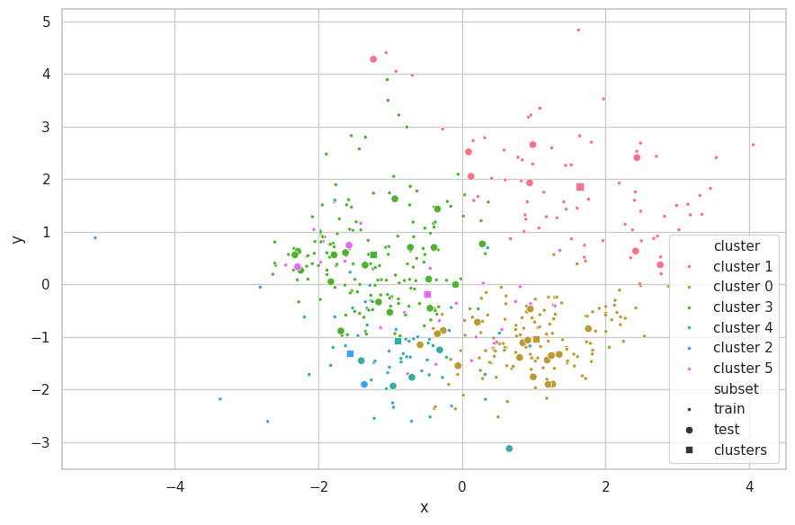
visualize_clusters(
  (cluster_train, p_train, 'train', '.'),
  (cluster_test, p_test, 'test', 'o'),
  (clusters, p_clusters, 'clusters', 's')
)
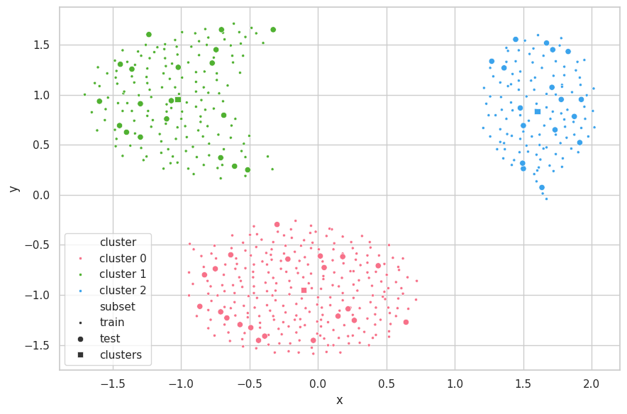
Discussions
The search strategy found the correct underlying structure of the data ($K=3$). With it, K-Means was able to perfecly separate the data. The centroids of the clusters are seemly positioned on the center of each data mass.
As the train-test subsets were split through random selection, the data distributions from these sets are fairly similar. Therefore, the K-Means produced similar results for all metrics associated (WCSS, BCSS and Silhouette).
A few points from the test set stand out, being the fartherest from the centroid of their clusters (bottom samples of clusters 1 and 2). For cluster 1, two samples are close to the decision boundary between cluster 0 and 1, in which each is assigned a different label. As for cluster 2, the three outlying samples are still correctly labeled. Further inspection — and information around the problem domain — is needed in order to verify if these samples are indeed exceptional cases or merely noise during the capturing procedure.
Application over The California Dataset
Searching K
%%time

report = kmeans_search(
  cali_x_train,
  k_max=Config.cali.k_max,
  steps=Config.cali.steps,
  repeats=Config.cali.repeats,
  verbose=2
)
k: 2, performing 100 tests
....................................................................................................
k: 3, performing 100 tests
....................................................................................................
k: 4, performing 100 tests
....................................................................................................
k: 5, performing 100 tests
....................................................................................................
k: 6, performing 100 tests
....................................................................................................
k: 7, performing 100 tests
....................................................................................................
k: 8, performing 100 tests
....................................................................................................
k: 9, performing 100 tests
....................................................................................................
k: 10, performing 100 tests
....................................................................................................
CPU times: user 12min 8s, sys: 2.56 s, total: 12min 11s
Wall time: 11min 44s
report.groupby('k').mean().round(2).T
| k | repetition | Loss | WCSS | BCSS | Silhouette | WC Silhouette | Samples |
|---|---|---|---|---|---|---|---|
| 2 | 49.5 | 2985.78 | 6.64 | 18.13 | 0.36 | 0.18 | [259.2, 190.8] |
| 3 | 49.5 | 2543.88 | 5.65 | 37.92 | 0.35 | 0.12 | [182.89, 133.99, 133.12] |
| 4 | 49.5 | 2270.23 | 5.04 | 69.53 | 0.37 | 0.09 | [141.5, 105.96, 95.41, 107.13] |
| 5 | 49.5 | 2052.74 | 4.56 | 91.41 | 0.37 | 0.07 | [109.45, 98.78, 91.96, 73.3, 76.51] |
| 6 | 49.5 | 1863.19 | 4.14 | 107.14 | 0.38 | 0.06 | [96.67, 78.08, 66.52, 67.57, 71.96, 69.2] |
| 7 | 49.5 | 1738.49 | 3.86 | 151.44 | 0.38 | 0.05 | [87.26, 70.27, 66.63, 57.43, 60.75, 54.7, 52.96] |
| 8 | 49.5 | 1621.18 | 3.60 | 160.81 | 0.35 | 0.04 | [71.36, 53.04, 58.04, 54.13, 53.49, 55.07, 54.... |
| 9 | 49.5 | 1534.87 | 3.41 | 201.23 | 0.35 | 0.04 | [68.72, 51.51, 53.42, 44.84, 51.37, 45.14, 47.... |
| 10 | 49.5 | 1459.060 | 3.24 | 218.63 | 0.33 | 0.03 | [63.48, 46.85, 43.4, 40.76, 44.69, 41.34, 40.2... |
plt.figure(figsize=(16, 3))
plt.subplot(141).set_title('Within-Cluster Avg Squared Error'); sns.lineplot(data=report, x='k', y='WCSS')
plt.subplot(142).set_title('Between-Cluster Sum Squared Error'); sns.lineplot(data=report, x='k', y='BCSS')
plt.subplot(143).set_title('Avg Silhouette'); sns.lineplot(data=report, x='k', y='Silhouette')
plt.subplot(144).set_title('Within-Cluster Avg Silhouette'); sns.lineplot(data=report, x='k', y='WC Silhouette')
plt.tight_layout();
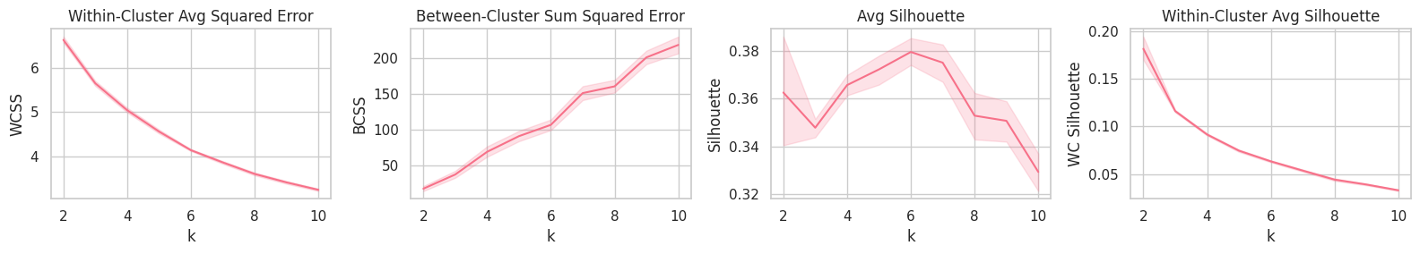
Training
Although the Avg. and Within-Cluster Avg. Silhouette curves point $k=6$ as the best (on average) parameter, WCSS and BCSS show that a large quantity of the system’s total distance error could still be transfered from the within-distance component to the between-distance one by increasing the $k$ parameter.
best_k = report.groupby('k').mean().Silhouette.idxmax()

print(f'Manually selected K: {best_k}')
Manually selected K: 6
clusters = tf.Variable(normal_clusters(cali_x_train, best_k), name=f'ck{best_k}')
clusters = kmeans_fit(
  cali_x_train,
  clusters,
  steps=Config.cali.steps,
  tol=Config.cali.tol,
  report_every=25,
  verbose=2
)
Step 0
  Loss          =     3919.007
  WCSS          =       8.7089
  BCSS          =      83.3113
  Silhouette    =       0.0903
  WC Silhouette =       0.0151
  Samples       = [126 132  15  97  50  30]
Step 25
  Loss          =    2086.1292
  WCSS          =       4.6358
  BCSS          =       75.879
  Silhouette    =       0.3722
  WC Silhouette =        0.062
  Samples       = [152  77  16 155  39  11]
Step 50
  Loss          =    1901.8014
  WCSS          =       4.2262
  BCSS          =      77.6798
  Silhouette    =       0.3968
  WC Silhouette =       0.0661
  Samples       = [144  73  13 148  45  27]
Step 75
  Loss          =     1824.202
  WCSS          =       4.0538
  BCSS          =      80.4515
  Silhouette    =       0.4082
  WC Silhouette =        0.068
  Samples       = [141  71  11 152  49  26]
Step 100
  Loss          =    1794.4468
  WCSS          =       3.9877
  BCSS          =      84.4598
  Silhouette    =       0.4106
  WC Silhouette =       0.0684
  Samples       = [139  71  10 155  49  26]
Evaluation
p_train = kmeans_predict(cali_x_train, clusters)
p_test = kmeans_predict(cali_x_test, clusters)
p_clusters = tf.range(best_k)  # clusters tags are trivial: [0, 1, 2, ...]

kmeans_report_evaluation('Train', cali_x_train, clusters)
kmeans_report_evaluation('Test', cali_x_test, clusters)
Train
  Loss          =    1794.4468
  WCSS          =       3.9877
  BCSS          =      84.4598
  Silhouette    =       0.4106
  WC Silhouette =       0.0684
  Samples       = [139  71  10 155  49  26]
Test
  Loss          =      189.131
  WCSS          =       3.7826
  BCSS          =      81.9574
  Silhouette    =       0.4865
  WC Silhouette =       0.0811
  Samples       = [16  8  1 18  5  2]
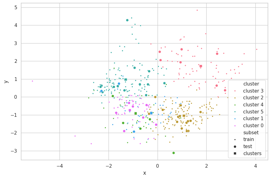
e = PCA(n_components=2)

visualize_clusters(
  (e.fit_transform(cali_x_train, p_train), p_train, 'train', '.'),
  (e.transform(cali_x_test), p_test, 'test', 'o'),
  (e.transform(clusters), p_clusters, 'clusters', 's')
)
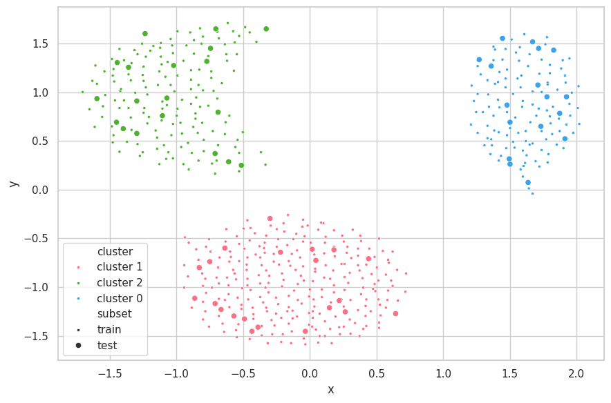
Discussions
We are limited by the number of attributes that can be plotted at the same time in a scatterplot. Considering the California Dataset has more than two features, not all information is shown in the chart above. We opted to use PCA [6] as a visualization method to select the directions of most variability in the assignment of clusters and further improve the visualization. We remark that this step is performed after K-Means execution, and therefore does not affect the results of the clustering method.
From the scatterplot above, we observe this set represents a much more complex structure than the Cluster.dat Dataset.
Application over The TF-Flowers Dataset
Preparing
In order to use K-Means, as implemented above, we transform our image dataset into a feature-vector dataset. Furthermore, we “normalize” the samples features (pixels) by compressing their RGB values $[0, 256)$ into the $[-1, 1]$ interval.
def preprocess_input(x):
  x = tf.reshape(x, (-1, Config.tf_flowers.channels))
  x /= 127.5
  x -= 1
  return x

def postprocess_output(z):
  z += 1
  z *= 127.5
  z = tf.reshape(z, (-1, *Config.tf_flowers.shape))
  return z
Training
for flowers_train, _ in flowers_train_set.take(1):
  flowers_train = preprocess_input(flowers_train)  # (8, 150, 150, 3) -> (180,000, 3)

  s = tf.random.uniform([Config.tf_flowers.training_samples],
                        maxval=flowers_train.shape[0],
                        dtype=tf.int32)
  flowers_train_selected = tf.gather(flowers_train, s, axis=0)  # (10,000, 3)

clusters = tf.Variable(uniform_clusters(
  flowers_train,
  Config.tf_flowers.colors
))
visualize_images(
  tf.reshape(tf.cast(127.5*(clusters + 1), tf.int32), (1, 4, -1, 3)),
  figsize=(6, 2),
  rows=1)

%%time

try: clusters = kmeans_fit(
       flowers_train_selected,
       clusters,
       steps=Config.tf_flowers.steps,
       tol=Config.tf_flowers.tol,
       verbose=2)
except KeyboardInterrupt: print('\ninterrupted')
else: print('done')

# Constrain to valid image pixel values.
clusters.assign(tf.clip_by_value(clusters, -1., 1.));
Step 0
  Loss          =     711.2058
  WCSS          =       0.0711
  BCSS          =      295.279
  Silhouette    =      -0.9991
  WC Silhouette =      -0.0078
  Samples       = [ 28   4   0   3   0  20  68   0  15 382   0   0 215   0  12   0  24   2
  10  22 187   0   0   2 198   9   1   0   2   0 397   0  98   0  58  59
  17  82   0   0 114   0   0   0 941   0   1   0  12 116   0 423   0   1
   0 118 107   0   0 237   0   0 114   4 894  30 533   1   0 290 594   0
   0   0  17  85   0   1 177  55   7  14   1   5   0   0   0   0   0  50
   0  42   0   0   9  15   7   7  26 116  12   0 123   0   1   0   0  99
  40 174 355  23   1   0 871 141 385 521   0  14  12   0  68   1  42   0
   0  38]
Step 10
  Loss          =     260.2131
  WCSS          =        0.026
  BCSS          =     296.0636
  Silhouette    =      -0.9991
  WC Silhouette =      -0.0078
  Samples       = [ 32   6   0   1   0   6  60   0  11 308   0   0 336   0  12   0  36   1
   7  24 140   0   0   4 164   8   1   0   2   0 321   4 225   0  75  46
  21 136   0   0 114   0   0   0 338   0   1   0  11 327   0 225   0   0
   0 154 147   0   0 237   0   0 104   4 488  34 336   0   0 262 599   0
   0   0  24 116   0  10 179  59   6  19   1   7   0   0   0   0   0  80
   0 155   0   0 100   3  20   6  49 116  13   2 141   1   1   0   0 309
  41 180 738   3   1   0 812 320 414 475   0  32  28   0  87   1  43   0
   0  40]
Step 20
  Loss          =     223.4796
  WCSS          =       0.0223
  BCSS          =     296.1174
  Silhouette    =      -0.9992
  WC Silhouette =      -0.0078
  Samples       = [ 32   6   0   1   0   7  64   0  12 217   0   0 290   0  19   0  63   1
   5  33 120   0   0  11 149   8   1   0   2   0 281   0 218   0  89 203
  19 145   0   0 131   0   0   0 284   0   2   0  10 370   0 207   0   0
   0 163 149   0   0 244   0   0 106   5 487  35 294   0   0 250 543   0
   0   0  20 116   0  31 192 108   6  24   1   8   0   0   0   0   0  81
   0 196   0   0 178   3  34   6  60 118  10   2 138   1   1   0   0 238
  42 207 655   4   1   0 796 266 405 419   0  60  55   0 156   1  44   0
   0  41]
Step 30
  Loss          =     208.6662
  WCSS          =       0.0209
  BCSS          =     296.3314
  Silhouette    =      -0.9993
  WC Silhouette =      -0.0078
  Samples       = [ 31   8   0   1   0   7  68   0  13 182   0   0 288   0  24   0  70   0
   4  43 120   0   0  12 138   8   1   0   3   0 301   0 201   0  90 402
  18 129   0   0 180   0   0   0 178   0   2   0  10 349   0 184   0   0
   0 143 144   0   0 233   0   0 103   5 466  41 291   0   0 253 542   0
   0   0  17 110   0  56 180 129   6  26   1   9   0   0   0   0   0  89
   0 206   0   0 181   3  57   6  73 121   9   2 136   1   1   0   0 229
  42 221 616   4   1   0 781 245 401 368   0  74  67   0 162   1  44   0
   0  39]
Step 40
  Loss          =     202.2344
  WCSS          =       0.0202
  BCSS          =      296.567
  Silhouette    =      -0.9994
  WC Silhouette =      -0.0078
  Samples       = [ 29   8   0   1   0   7  71   0  13 176   0   0 293   0  24   0  79   0
   4  56 127   0   0  23 138   9   1   0   3   0 307   0 194   0  91 519
  18 127   0   0 191   0   0   0 170   0   2   0  12 337   0 175   0   0
   0 137 136   0   0 227   0   0 104   5 449  45 284   0   0 254 537   0
   0   0  22 113   0  72 167 134   6  27   1   9   0   0   0   0   0  90
   0 214   0   0 171   3  75   6  78 121   9   2 123   1   2   0   0 225
  43 215 539   4   1   0 712 235 403 390   0  88  76   0 154   1  46   0
   0  39]
Step 50
  Loss          =       198.52
  WCSS          =       0.0199
  BCSS          =     296.7816
  Silhouette    =      -0.9993
  WC Silhouette =      -0.0078
  Samples       = [ 29   8   0   1   0   7  76   0  14 173   0   0 288   0  25   0  84   0
   4  64 136   0   0  40 140  10   1   0   4   0 300   0 183   0  92 538
  18 127   0   0 195   0   0   0 165   0   1   0  12 327   0 169   0   0
   0 131 129   0   0 224   0   0 102   7 428  48 258   0   0 249 552   0
   0   0  29 118   0  94 165 142   6  29   1   9   0   0   0   0   0  86
   0 222   0   0 173   3  83   6  80 119   9   2 116   1   2   0   0 224
  43 218 535   5   1   0 687 224 398 395   0  96  85   0 148   1  46   0
   0  40]
Step 60
  Loss          =     195.9817
  WCSS          =       0.0196
  BCSS          =     296.8312
  Silhouette    =      -0.9993
  WC Silhouette =      -0.0078
  Samples       = [ 28  10   0   1   0   7  84   0  14 173   0   0 292   0  26   0  80   0
   4  63 140   0   0  65 143  10   1   0   4   0 297   0 176   0  94 522
  19 133   0   0 192   0   0   0 156   0   1   0  13 307   0 167   0   0
   0 127 127   0   0 217   0   0 102   8 401  49 251   0   0 245 564   0
   0   0  46 115   0 126 164 148   6  31   1   9   0   0   0   0   0  85
   0 224   0   0 169   3  82   6  81 119  10   4 116   1   2   0   0 223
  43 218 550   5   1   0 685 219 397 387   0  96  89   0 137   1  46   0
   0  42]
Step 70
  Loss          =     193.5877
  WCSS          =       0.0194
  BCSS          =      296.789
  Silhouette    =      -0.9993
  WC Silhouette =      -0.0078
  Samples       = [ 25  10   0   1   0   6  89   0  15 173   0   0 283   0  26   0  78   0
   6  64 134   0   0  91 142  11   1   0   4   0 288   0 170   0  95 517
  19 141   0   0 191   0   0   0 154   0   1   0  16 307   0 171   0   0
   0 137 125   0   0 215   0   0 102  10 371  50 242   0   0 239 569   0
   0   0  59 115   0 164 159 151   7  33   1  10   0   0   0   0   0  85
   0 233   0   0 161   3  80   6  82 117   9   4 111   1   2   0   0 223
  42 220 551   8   1   0 684 210 402 381   0  83  95   0 127   1  47   0
   0  43]
Step 80
  Loss          =     191.9187
  WCSS          =       0.0192
  BCSS          =     296.7511
  Silhouette    =      -0.9992
  WC Silhouette =      -0.0078
  Samples       = [ 24  11   0   1   0   6  88   0  16 174   0   0 284   0  27   0  78   0
   9  65 136   0   0 107 142  11   1   0   4   0 279   0 166   0  93 510
  22 150   0   0 195   1   0   0 151   0   1   0  17 301   0 171   0   0
   0 140 123   0   0 219   0   0 102  10 349  54 242   0   0 235 561   0
   0   0  65 115   0 197 155 150   7  31   1  13   0   0   0   0   0  86
   0 239   0   0 169   3  78   6  81 116   9   4 108   1   2   0   0 219
  43 216 550   9   1   0 687 201 398 378   0  80  92   0 118   1  49   0
   0  46]
Step 90
  Loss          =      190.467
  WCSS          =        0.019
  BCSS          =     296.7254
  Silhouette    =      -0.9992
  WC Silhouette =      -0.0078
  Samples       = [ 24  11   0   1   0   6  89   0  16 174   0   0 278   0  27   0  81   0
  18  64 127   0   0 124 142  11   1   0   4   0 267   0 160   0  93 510
  24 153   0   0 201   1   0   0 151   0   1   0  17 300   0 171   0   0
   0 144 123   0   0 217   0   0 102  10 342  58 242   0   0 242 558   0
   0   0  67 114   0 213 154 150   7  31   1  14   0   0   0   0   0  88
   0 231   0   0 176   3  81   6  80 115   9   5 105   1   2   0   0 215
  41 218 550  12   1   0 687 193 389 373   0  75  94   0 116   1  50   0
   0  47]
Step 100
  Loss          =     188.9857
  WCSS          =       0.0189
  BCSS          =     296.6828
  Silhouette    =      -0.9992
  WC Silhouette =      -0.0078
  Samples       = [ 23  11   0   1   0  10  91   0  18 177   0   0 275   0  27   0  82   0
  24  62 137   0   0 129 141  11   1   0   4   0 261   0 158   0  90 503
  25 154   0   0 198   1   0   0 148   0   1   0  17 286   0 170   0   0
   0 151 119   0   0 216   0   0 102  11 327  60 237   0   0 247 540   0
   0   0  67 111   0 239 153 150   8  39   1  15   0   0   0   0   0  89
   0 231   0   0 209   3  82   6  79 112   9   5 101   1   2   0   0 216
  40 220 545  16   1   0 687 183 384 369   0  73  96   0 113   1  51   0
   0  47]
done
CPU times: user 3min 40s, sys: 27.3 s, total: 4min 7s
Wall time: 2min 32s
visualize_images(
  tf.reshape(tf.cast(127.5*(clusters + 1), tf.int32), (1, 4, -1, 3)),
  figsize=(6, 2),
  rows=1)

Transforming Images
Images are encoded by replacing each pixel in the images by its cluster index (three 32-bit floating numbers are replaced by an 32-bit integer), and reconstructed by replacing the cluster index by the cluster point itself.
for x, _ in flowers_test_set.take(3):
  # Encoding:
  y = kmeans_predict(preprocess_input(x), clusters)

  print(f'Encoding {x.shape[0]} images:')
  print(f'  shape: {x.shape} to {y.shape}')
  print(f'  size:  {size_in_mb(x):.2f} MB to {size_in_mb(y):.2f} MB')

  # Decoding:
  z = tf.gather(clusters, y, axis=0)
  z = postprocess_output(z)

  visualize_images([*tf.cast(x, tf.uint32), *tf.cast(z, tf.uint32)], figsize=(16, 4))
  plt.subplots_adjust(wspace=0, hspace=0)
Encoding 8 images:
  shape: (8, 150, 150, 3) to (180000,)
  size:  4.12 MB to 1.37 MB
Encoding 8 images:
  shape: (8, 150, 150, 3) to (180000,)
  size:  4.12 MB to 1.37 MB
Encoding 8 images:
  shape: (8, 150, 150, 3) to (180000,)
  size:  4.12 MB to 1.37 MB
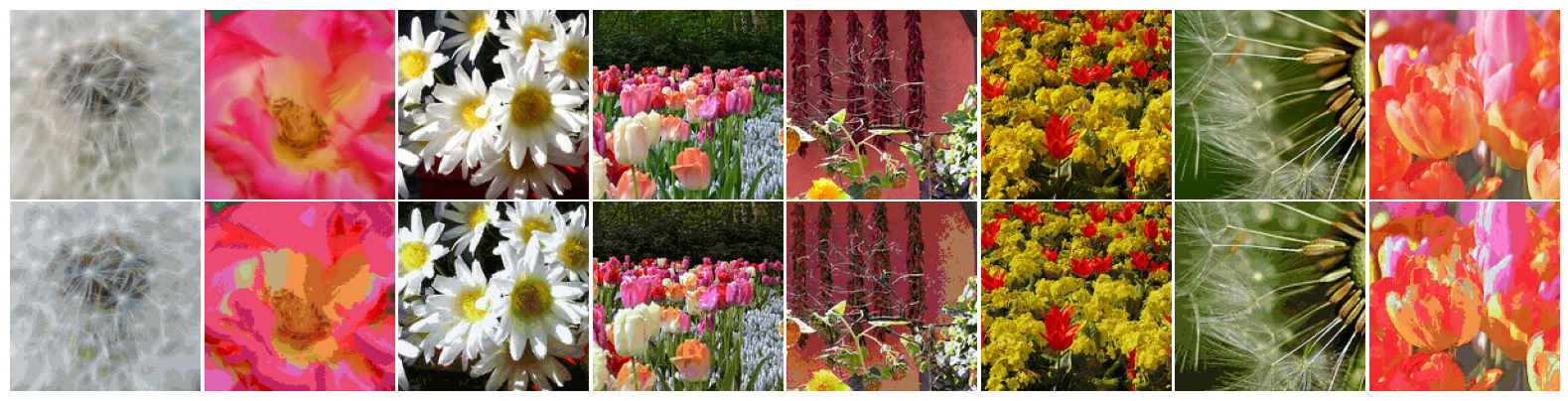
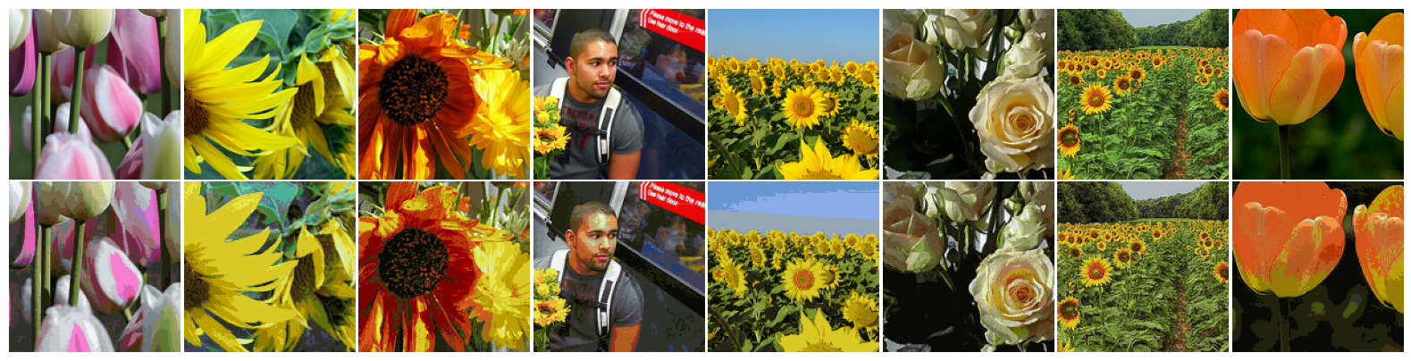
Discussions
Using this strategy, each $(150, 150, 3)$ image can be encoded into a $22500$-d vector. Memory requirements for storing this information is reduced to 33.25% (0.52 MB to 0.17 MB), plus the color code-book (global to the entire set).
Considering only the 24 test samples above, details seem to have been correctly preserved in all images. Conversely, smooth sections of the images containing gradual color shift were most impacted by the compression process.
Efficacy could be improved by using more images from multiple batches.
Hierarchical Clustering
We implemented the bottom-up strategy for Hierarchical Clustering [7]. This algorithm relies heavily on the greedy linkage between two shortest-distant clusters.
In order to efficiently perform this operation, a few assumptions are made:
- The distance between each pair of points in the set does not change after the algorithm starts. Hence the distance matrix is computed only once.
- Linkage between clusters
aandbis the same as the linkage betweenbanda. I.e., linkage behaves as a distance function. - The
heapqmodule holds an efficient handling for heap/priority queues (which is true, considering our empirical results)
We start by implementing the ClusterQueue class.
When instantiated, an object of ClusterQueue receives as arguments a sample-wise distance matrix, a list of clusters (usually singletons) and a linkage function.
The heap ClusterQueue#pq is then built using each $\binom{|C|}{2}$ pair of clusters (and their linkage).
Two methods are now available: (1) pop, which retrieves the two closest clusters (according to their linkage) and (2) merge, which takes two clusters as arguments, merge them and add them to the heap.
During testing, the linkage between each sample in the test set is computed to each cluster in the training set, resulting in a cluster assignment (label) for each test sample.
Algorithm
import heapq


class ClusterQueue:
  """Priority Queue for sets of points (clusters).

  Arguments
  ---------
  distance: np.ndarray
    distance matrix between each pair of samples in the training data

  clusters: list of list of ints
    Starting configuration of clusters.
    Generally starts with singletons [[0], [1], [2], ...]

  linkage: str
    Linkage function used when computing distance between two clusters.

  """

  def __init__(self, distances, clusters, linkage):
    self.d = distances
    self.clusters = clusters
    self.linkage = get_linkage_by_name(linkage)

    self.build()

  def build(self):
    """Builds the priority queue containing elements (dist(a, b), a, b).
    """
    pq = []

    for i, a in enumerate(self.clusters):
      for j in range(i+1, len(self.clusters)):
        b = self.clusters[j]
        d_ab = self.linkage(self.d[a][:, b])
        pq.append((d_ab, a, b))

    heapq.heapify(pq)
    self.pq = pq

  def pop(self):
    # Invalid links (between old clusters) might exist as we merge
    # and create new clusters. Continue until we find a valid one.
    while True:
      d, a, b = heapq.heappop(self.pq)

      if a in self.clusters and b in self.clusters:
        return d, a, b

  def merge(self, a, b):
    # Removes `a` and `b` from `clusters`, adds the distances
    # `d(c, o), for all o in clusters` to the priority queue.
    # Finally, adds a new set `c=a+b`.
    self.clusters.remove(a)
    self.clusters.remove(b)

    c = a + b

    for o in self.clusters:
      d_co = self.linkage(self.d[c][:, o])
      heapq.heappush(self.pq, (d_co, c, o))

    self.clusters.append(c)
from scipy.spatial.distance import cdist


def hierarchical_clustering(
    x: np.ndarray,
    metric: str = 'euclidean',
    linkage: str = 'average',
    max_e: float = None,
    min_k: int = 2,
    max_steps: int = None,
    verbose: int = 1,
    report_every: int = 50
) -> List[List[int]]:
  """Hierarchical Clustering.

  Arguments
  ---------
  x: np.ndarray
    Training data.
  metric: str
    Passed to `scipy.spatial.distance.cdist`. Metric used when computing
    distances between each pair of samples. Options are:
      braycurtis, canberra, chebyshev, cityblock, correlation,
      cosine, dice, euclidean, hamming, jaccard, jensenshannon,
      kulsinski, mahalanobis, matching, minkowski, rogerstanimoto,
      russellrao, seuclidean, sokalmichener, sokalsneath, sqeuclidean,
      wminkowski, yule
  linkage: Callable
    Cluster linkage strategy. Options are:
      average, single, complete
  max_e: float
    Maximum linkage that is still considered as "close". Early stopping threshold.
  min_k: int
    Minimum number of clusters before stopping. Early stopping threshold.
  max_steps: int
    Maximum number of iterations allowed. early stopping threshold.
  verbosity:
    Controls the process verbosity. Options are 0, 1 or 2.
  report_every:
    Controls how frequently evaluation is performed.

  Returns
  -------
  List of set of point indices.
    A list containing the clustered points found.
    Each element of the list is a set of indices for the first axis of the training data:

    x := [[x00, x01, x02, ...],
          [x10, x11, x12, ...],
          ... ]

    hierarchical_clustering(x, ...)
      := [[0, 4, 5], [1, 2, 6], [3, 7, 10], ...]
  """
  cq = ClusterQueue(distances=cdist(x, x, metric=metric),
                    clusters=[[i] for i in range(len(x))],
                    linkage=linkage)
  step = 1

  while len(cq.clusters) > 1:
    d_ab, a, b = cq.pop()

    if verbose > 1 and step % report_every == 0:
      hc_report_evaluation(f'Step {step}', x, x, cq.clusters, metric, linkage, d=cq.d)

    if max_e and d_ab > max_e:
      if verbose: print(f'\nEarly stopping: shortest linkage > max_e [{d_ab:.4f} > {max_e:.4f}]')
      break
    if len(cq.clusters) <= min_k:
      if verbose: print(f'\nEarly stopping: k <= min_k [{len(cq.clusters)} <= {min_k}]')
      break
    if max_steps and step >= max_steps:
      if verbose: print(f'\nEarly stopping: steps >= max_steps set [{step} >= {max_steps}]')
      break

    cq.merge(a, b)
    step += 1

  if verbose == 1 or verbose > 1 and step % report_every:
    # last step, if not reported yet.
    hc_report_evaluation(f'Step {step}', x, x, cq.clusters, metric, linkage, d=cq.d)

  return cq.clusters


def hc_report_evaluation(tag, s, x, clusters, metric, linkage, d=None):
  report = hc_test_step(s, x, clusters, metric, linkage, d=d)

  print(tag)
  lpad = max(map(len, report)) + 2
  rpad = 12

  for metric, value in report.items():
    print(f'  {metric}'.ljust(lpad), '=', str(np.round(value, 4)).rjust(rpad))


def hc_test_step(
    s: np.asarray,
    x: np.asarray,
    clusters: List[List[int]],
    metric: str = 'euclidean',
    linkage: str = 'average',
    d: np.asarray = None
) -> Dict[str, float]:
  if d is None:  # Reuse distance matrix if it was already computed.
    d = cdist(s, x, metric=metric)

  linkage = get_linkage_by_name(linkage)

  # Samples in the training set `x` have trivial labels.
  yx = np.zeros(len(x))
  for ix, c in enumerate(clusters): yx[c] = ix

  # Calculate labels in sample set `s`.
  ys = [linkage(d[:, c], axis=1) for c in clusters]
  ys = np.argmin(ys, axis=0)

  samples = HCMetrics.samples_per_cluster(ys)
  wss_ = HCMetrics.WCSS(d, ys, yx, linkage)
  bss_ = HCMetrics.BCSS(d, ys, yx, linkage)
  sil_ = HCMetrics.silhouette(d, ys, yx, linkage)
  wc_sil_ = HCMetrics.wc_avg_silhouette(d, ys, yx, linkage)

  return dict(zip(
    ('Loss', 'WCSS', 'BCSS', 'Silhouette', 'WC Silhouette', 'Clusters', 'Samples'),
    (np.sum(np.concatenate(wss_)),
     np.mean(np.concatenate(wss_)),
     np.mean(np.concatenate(bss_)),
     np.mean(sil_),
     np.mean(wc_sil_),
     len(clusters),
     samples[:10])
  ))
def hc_search(
  x: np.ndarray,
  params: Union[List[Dict[str, Any]], ParameterGrid],
  max_steps: int = None,
  verbose: int = 1,
) -> pd.DataFrame:
  """Search for Hyper-Parameter Optimization.

  Returns
  -------
    pd.DataFrame
      The search results report.
  """
  results = []

  for ix, p in enumerate(params):
    if verbose > 0: print(f'params: {p}')

    clusters = hierarchical_clustering(x, max_steps=max_steps, verbose=0, **p)
    metrics = hc_test_step(x, x, clusters, p['metric'], p['linkage'])
    results += [{'config_id': ix, 'params': p, **metrics}]

  return pd.DataFrame(results)
def hc_predict(
  s: np.ndarray,
  x: np.ndarray,
  clusters: List[List[int]],
  metric: str = 'euclidean',
  linkage: str = 'average',
) -> np.array:
  """Hierarchical Clustering Predict.

  Predict new samples based on minimal distance to existing clusters,
  without altering their current configuration.

  """
  d = cdist(s, x, metric=metric)
  linkage = get_linkage_by_name(linkage)

  # We need a label for every single point, so we calculate
  # single point-to-cluster distance (hence axis=1).
  l = [linkage(d[:, c], axis=1) for c in clusters]
  l = np.argmin(l, axis=0)

  return l
Linkage and Evaluation Metrics
def single_linkage(d, axis=None):
  return np.min(d, axis=axis)

def average_linkage(d, axis=None):
  return np.mean(d, axis=axis)

def complete_linkage(d, axis=None):
  return np.max(d, axis=axis)


def get_linkage_by_name(name):
  return globals()[f'{name}_linkage']


# Metrics

class HCMetrics:
  @staticmethod
  def WCSS(d, yx, yc, linkage, reducer=None):
    return [linkage(d[yx == label][:, yc == label], axis=1) for label in np.unique(yx)]

  @staticmethod
  def BCSS(d, yx, yc, linkage, reducer=np.concatenate):
    return [linkage(d[yx == label][:, yc != label], axis=1) for label in np.unique(yx)]

  @staticmethod
  def silhouette(d, yx, yc, linkage):
    a = np.concatenate(HCMetrics.WCSS(d, yx, yc, linkage))
    b = np.concatenate(HCMetrics.BCSS(d, yx, yc, linkage))

    return (b - a) / np.maximum(a, b)

  @staticmethod
  def wc_avg_silhouette(d, yx, yc, linkage):
    # WCSS and BCSS return tensors in the shape (clusters, samples),
    # so we can simply zip them together:
    return np.asarray([
      np.mean((b-a) / np.maximum(a, b))
      for a, b in zip(HCMetrics.WCSS(d, yx, yc, linkage),
                      HCMetrics.BCSS(d, yx, yc, linkage))
    ])

  @staticmethod
  def samples_per_cluster(yx):
    return np.unique(yx, return_counts=True)[1]
Application over The Cluster.dat Dataset
Searching
%%time

report = hc_search(
  cluster_train.numpy(),
  params=ParameterGrid({
    'metric': ['euclidean'],    # ... 'correlation'] --- different metrics aren't directly comparable.
    'linkage': ['average'],   # ... 'average', 'complete'] --- different linkages aren't directly comparable.
    'max_e': [.4, .5, .6, .7, .8, .9, 1.],
    'min_k': [3]
  }),
  max_steps=1000,
  verbose=1
).set_index('config_id').round(2)
params: {'linkage': 'average', 'max_e': 0.4, 'metric': 'euclidean', 'min_k': 3}
params: {'linkage': 'average', 'max_e': 0.5, 'metric': 'euclidean', 'min_k': 3}
params: {'linkage': 'average', 'max_e': 0.6, 'metric': 'euclidean', 'min_k': 3}
params: {'linkage': 'average', 'max_e': 0.7, 'metric': 'euclidean', 'min_k': 3}
params: {'linkage': 'average', 'max_e': 0.8, 'metric': 'euclidean', 'min_k': 3}
params: {'linkage': 'average', 'max_e': 0.9, 'metric': 'euclidean', 'min_k': 3}
params: {'linkage': 'average', 'max_e': 1.0, 'metric': 'euclidean', 'min_k': 3}
CPU times: user 37.1 s, sys: 356 ms, total: 37.5 s
Wall time: 37.6 s
| config_id | params | Loss | WCSS | BCSS | Silhouette | WC Silhouette | Clusters | Samples |
|---|---|---|---|---|---|---|---|---|
| 0 | {'linkage': 'average', 'max_e': 0.4, 'metric':... | 123.15 | 0.24 | 1.83 | 0.87 | 0.87 | 22 | [18, 21, 19, 17, 12, 26, 26, 24, 15, 26] |
| 1 | {'linkage': 'average', 'max_e': 0.5, 'metric':... | 172.52 | 0.33 | 1.90 | 0.82 | 0.82 | 12 | [23, 35, 51, 29, 32, 47, 27, 60, 59, 40] |
| 2 | {'linkage': 'average', 'max_e': 0.6, 'metric':... | 188.88 | 0.37 | 1.92 | 0.80 | 0.81 | 10 | [27, 34, 47, 72, 59, 44, 69, 54, 64, 46] |
| 3 | {'linkage': 'average', 'max_e': 0.7, 'metric':... | 210.21 | 0.41 | 1.96 | 0.78 | 0.79 | 8 | [35, 88, 59, 56, 54, 73, 60, 91] |
| 4 | {'linkage': 'average', 'max_e': 0.8, 'metric':... | 271.66 | 0.53 | 2.10 | 0.74 | 0.75 | 5 | [48, 121, 131, 113, 103] |
| 5 | {'linkage': 'average', 'max_e': 0.9, 'metric':... | 334.00 | 0.65 | 2.39 | 0.72 | 0.73 | 3 | [113, 252, 151] |
| 6 | {'linkage': 'average', 'max_e': 1.0, 'metric':... | 334.00 | 0.65 | 2.39 | 0.72 | 0.73 | 3 | [113, 252, 151] |
Training
%%time

params = dict(
  metric='euclidean',
  linkage='average',
  max_e=.9,
)

clusters = hierarchical_clustering(
  cluster_train.numpy(),
  **params,
  max_steps=1000,
  report_every=250,
  verbose=2
)
Step 250
  Loss          =      17.0699
  WCSS          =       0.0331
  BCSS          =       1.7615
  Silhouette    =       0.9805
  WC Silhouette =       0.9852
  Clusters      =          267
  Samples       = [1 1 1 1 1 1 1 1 1 1]
Step 500
  Loss          =     143.1246
  WCSS          =       0.2774
  BCSS          =       1.8524
  Silhouette    =       0.8452
  WC Silhouette =       0.8511
  Clusters      =           17
  Samples       = [16 26 30 26 35 35 28 30 35 25]

Early stopping: shortest linkage > max_e [2.1811 > 0.9000]
Step 514
  Loss          =     333.9982
  WCSS          =       0.6473
  BCSS          =       2.3875
  Silhouette    =       0.7229
  WC Silhouette =       0.7328
  Clusters      =            3
  Samples       = [113 252 151]
CPU times: user 6.54 s, sys: 36.8 ms, total: 6.57 s
Wall time: 6.72 s
Evaluate
p_train = hc_predict(cluster_train.numpy(), cluster_train.numpy(), clusters,
                     params['metric'], params['linkage'])
p_test = hc_predict(cluster_test.numpy(), cluster_train.numpy(), clusters,
                    params['metric'], params['linkage'])
visualize_clusters(
  (cluster_train, p_train, 'train', '.'),
  (cluster_test, p_test, 'test', 'o'),
)
Discussions
We assume multiple distances and linkages are not directly comparable, considering their differences in construction. For example, single linkage will always return lower values than average and complete linkage. Therefore, we only searched within a single combination of metric and linkage.
For Hierarchical Clustering, WCSS is minimal when all clusters are singleton, and will increase as the algorithm progresses. BCSS also increases as samples in the set are aggregated into fewer clusters, as their centroids become increasingly more distant from each other.
Furthermore, as the within cluster linkage tends to 0, max(a, b) tends to b, and the Silhouette tends to 1. As the algorithm executes, increasing a, the Avg. Silhouette decreases.
We were limited to search for the max_e and min_k parameters. As these are early stopping arguments and will dictate for how many iterations the algorithm will run, it becomes clear that larger max_e/lower min_k will always result in lower Avg. Silhouette values.
Therefore, we selected the winning searching arguments based on how many clusters they would produce, as well as the amount of samples in each cluster.
The Cluster.dat Dataset was once again easily clustered using $e=0.9$. The algorithm early stopped with the min distance threshold ($min(d) = 2.1811 > e=0.9$), and have correctly found the 3 clusters for the set.
Application over The California Dataset
Searching
%%time

report = hc_search(
  cali_x_train.numpy(),
  params=ParameterGrid({
    'metric': ['euclidean'],
    'linkage': ['average'],
    'max_e': [3., 4., 5., 6.],
  }),
  max_steps=1000,
  verbose=1
).set_index('config_id').round(2)
params: {'linkage': 'average', 'max_e': 3.0, 'metric': 'euclidean'}
params: {'linkage': 'average', 'max_e': 4.0, 'metric': 'euclidean'}
params: {'linkage': 'average', 'max_e': 5.0, 'metric': 'euclidean'}
params: {'linkage': 'average', 'max_e': 6.0, 'metric': 'euclidean'}
CPU times: user 17.3 s, sys: 152 ms, total: 17.4 s
Wall time: 17.5 s
| config_id | params | Loss | WCSS | BCSS | Silhouette | WC Silhouette | Clusters | Samples |
|---|---|---|---|---|---|---|---|---|
| 0 | {'linkage': 'average', 'max_e': 3.0, 'metric':... | 906.72 | 2.01 | 4.01 | 0.48 | 0.70 | 26 | [1, 4, 1, 1, 2, 1, 1, 1, 1, 1] |
| 1 | {'linkage': 'average', 'max_e': 4.0, 'metric':... | 1255.36 | 2.79 | 4.54 | 0.37 | 0.64 | 14 | [1, 1, 1, 6, 3, 1, 1, 2, 7, 20] |
| 2 | {'linkage': 'average', 'max_e': 5.0, 'metric':... | 1510.53 | 3.36 | 7.56 | 0.55 | 0.55 | 7 | [1, 20, 3, 8, 6, 2, 410] |
| 3 | {'linkage': 'average', 'max_e': 6.0, 'metric':... | 1510.53 | 3.36 | 7.56 | 0.55 | 0.55 | 7 | [1, 20, 3, 8, 6, 2, 410] |
Training
%%time

params = dict(
  metric='euclidean',
  linkage='average',
  max_e=5.
)

clusters = hierarchical_clustering(
  cali_x_train.numpy(),
  **params,
  max_steps=1000,
  report_every=100,
  verbose=2
).set_index("config_id")
Step 100
  Loss          =       65.996
  WCSS          =       0.1467
  BCSS          =        3.681
  Silhouette    =       0.9552
  WC Silhouette =       0.9769
  Clusters      =          351
  Samples       = [1 1 1 1 1 1 1 1 1 1]
Step 200
  Loss          =     175.0656
  WCSS          =        0.389
  BCSS          =       3.6891
  Silhouette    =       0.8829
  WC Silhouette =       0.9413
  Clusters      =          251
  Samples       = [1 1 1 1 1 1 1 1 1 1]
Step 300
  Loss          =     341.0692
  WCSS          =       0.7579
  BCSS          =       3.7056
  Silhouette    =       0.7775
  WC Silhouette =       0.8766
  Clusters      =          151
  Samples       = [1 1 1 1 2 1 1 1 1 1]
Step 400
  Loss          =     704.2004
  WCSS          =       1.5649
  BCSS          =       3.8376
  Silhouette    =       0.5691
  WC Silhouette =       0.7321
  Clusters      =           51
  Samples       = [1 1 4 1 1 4 1 1 2 1]

Early stopping: shortest linkage > max_e [6.5662 > 5.0000]
Step 444
  Loss          =    1510.5264
  WCSS          =       3.3567
  BCSS          =       7.5577
  Silhouette    =       0.5474
  WC Silhouette =       0.5509
  Clusters      =            7
  Samples       = [  1  20   3   8   6   2 410]
CPU times: user 4.9 s, sys: 53.2 ms, total: 4.96 s
Wall time: 4.95 s
Evaluate
p_train = hc_predict(cali_x_train.numpy(), cali_x_train.numpy(), clusters, params['metric'], params['linkage'])
p_test = hc_predict(cali_x_test.numpy(), cali_x_train.numpy(), clusters, params['metric'], params['linkage'])
e = PCA(n_components=2)

visualize_clusters(
  (e.fit_transform(cali_x_train, p_train), p_train, 'train', '.'),
  (e.transform(cali_x_test), p_test, 'test', 'o'),
)
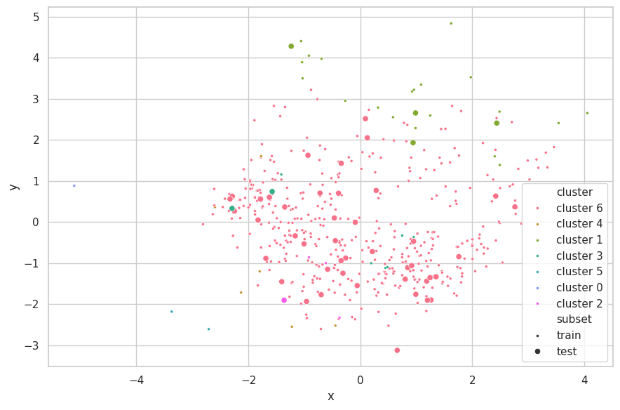
Discussions
We selected $e=5.0$, as this configuration resulted in 5 clusters more evenly balanced, with three seemly containing outliers. Greater values for $e$ resulted in a single main cluster being found, and two more containing few outlying samples.
The neighboring clusters found by K-Means have disapeared here. Furthermore, sparsely outlying samples have been clustered into small subsets (comprising of few samples). This confirms the search results found when applying the K-Means algorithm, which described this set as being dominated by two large clusters ($k=2$).
e = PCA(n_components=2)

z_train = e.fit_transform(cali_x_train)
z_test = e.transform(cali_x_test)

linkages = ('single', 'average', 'complete')
results = []


for linkage in linkages:
  clusters = hierarchical_clustering(
    cali_x_train.numpy(),
    metric='euclidean',
    linkage=linkage,
    max_e=4.,
    min_k=25,
    max_steps=1000,
    verbose=0)

  p_train = hc_predict(
    cali_x_train.numpy(),
    cali_x_train.numpy(),
    clusters,
    metric='euclidean',
    linkage=linkage)
  p_test = hc_predict(
    cali_x_test.numpy(),
    cali_x_train.numpy(),
    clusters,
    metric='euclidean',
    linkage=linkage)

  results += [(p_train, p_test)]


plt.figure(figsize=(12, 4))
for ix, (linkage, (p_train, p_test)) in enumerate(zip(linkages, results)):
  plt.subplot(1, 3, ix+1)
  visualize_clusters(
    (z_train, p_train, 'train', '.'),
    (z_test, p_test, 'test', 'o'),
    title=f'Hierarchical Clustering of California\nEuclidean {linkage} Linkage',
    full=False,
    legend=False
  )

plt.tight_layout()
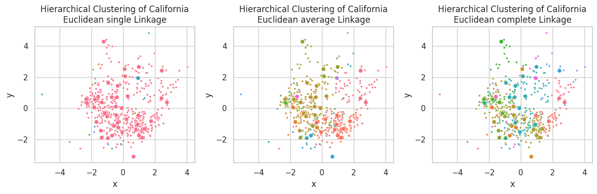
Single linkage is capable of finding non-linear relationships, where clusters are associated by their closest link, so non-spherical shaped clusters might appear (such as the pink one in the first plot). A downside of this linkage is the possible construction of unbalance clusters when data density varies across the space. This behavior can be observed in the California Dataset, were samples in the left-center are closely positioned, in opposite of the few samples on the right-bottom.
Complete linkage favors concise clusters in opposite of large ones, in which all samples are closely related. We observed for this example that the large data mass in the left-center was subdivided into multiple different clusters.
Average linkage seems as a compromise between Single and Complete linkage, pondering between cluster central similarity and sample conciseness.
Part-2: Dimensionality Reduction
How/if normalization affected our results
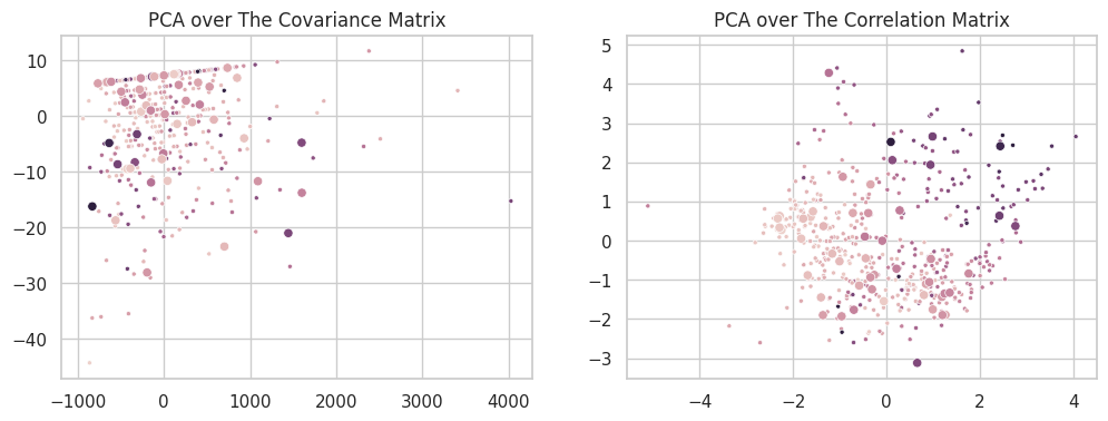
For a dataset $X$, where each feature is centered in $0$, Principal Component Analysis (PCA) can be expressed as the Singular Value Decomposition of the covariance matrix $XX^\intercal$ (which has the same sigular components as the matrix $X$). In a set of many features within different intervals, some features present larger variance intervals than others. In such cases, the sigular components will focus on modeling these directions, as their composition represent the highest total variance of the set. While this is interesting in many analytical cases, it is usually an unwanted behavior in Machine Learning: features should be favored based on how well they explain the overall data, independently of their natural variance.
A second formulation of the PCA can then be defined over the correlation matrix $\frac{XX^\intercal}{\sigma(X)^2}$. In this form, all features will vary in the same interval ($\mu_X=0, \sigma =1$), and the singular components will exclusively model the relationship between the variables. An easy way to achieve this form is to simply standardize the data (dividing each column by its standard deviation) before applying PCA. The new set will have $\sigma(X’)=1$ and its covariance and correlation matrices will be the same. The two scatterplots below show the difference between the two formulations on the California Dataset.
For the purposes of this assignment, all our PCA runs are based on the decomposition of the correlation matrix.
from sklearn.decomposition import PCA

e = PCA(n_components=2)

b_cov_train = e.fit_transform(inverse_standardize(cali_x_train, b_u, b_s))
b_cov_test = e.transform(inverse_standardize(cali_x_test, b_u, b_s))

b_cor_train = e.fit_transform(cali_x_train)
b_cor_test = e.transform(cali_x_test)
plt.figure(figsize=(12, 4))
plt.subplot(121)
plt.title('PCA over The Covariance Matrix')
sns.scatterplot(x=b_cov_train[:, 0], y=b_cov_train[:, 1], hue=cali_y_train, marker='.', label='train', legend=False)
sns.scatterplot(x=b_cov_test[:, 0], y=b_cov_test[:, 1], hue=cali_y_test, label='test', legend=False)

plt.subplot(122)
plt.title('PCA over The Correlation Matrix')
sns.scatterplot(x=b_cor_train[:, 0], y=b_cor_train[:, 1], hue=cali_y_train, marker='.', label='train', legend=False)
sns.scatterplot(x=b_cor_test[:, 0], y=b_cor_test[:, 1], hue=cali_y_test, label='test', legend=False)


del e, b_cov_train, b_cov_test, b_cor_train, b_cor_test
K-Means
Application over The California Dataset
energies = [0.5, .85, .9, .95, .99]
reductions = []

print(f'Data dimensionality: {cali_x_train.shape[1]}')

for energy in energies:
  e = PCA(n_components=energy)
  tr = e.fit_transform(cali_x_train)
  te = e.transform(cali_x_test)

  tr = tf.convert_to_tensor(tr, tf.float32)
  te = tf.convert_to_tensor(te, tf.float32)

  reductions.append((tr, te))

  print(f'Components used to explain e={energy:.0%}: {e.n_components_}')
Data dimensionality: 8
Components used to explain e=50.0%: 3
Components used to explain e=85.0%: 5
Components used to explain e=90.0%: 6
Components used to explain e=95.0%: 6
Components used to explain e=99.0%: 8
Searching K
%%time

report = pd.concat([
  kmeans_search(
    b,
    k_max=Config.cali.k_max,
    steps=Config.cali.steps,
    repeats=Config.cali.repeats,
    verbose=0
  ).assign(energy=e)
  for e, (b, _) in zip(energies, reductions)
])
CPU times: user 56min 28s, sys: 7.96 s, total: 56min 36s
Wall time: 54min 32s
report.drop(columns=["Samples"]).groupby("energy").mean().round(2)
| energy | k | repetition | Loss | WCSS | BCSS | Silhouette | WC Silhouette |
|---|---|---|---|---|---|---|---|
| 0.50 | 6.0 | 49.5 | 861.71 | 1.91 | 66.66 | 0.46 | 0.10 |
| 0.85 | 6.0 | 49.5 | 1653.47 | 3.67 | 98.63 | 0.39 | 0.08 |
| 0.90 | 6.0 | 49.5 | 1909.01 | 4.24 | 119.18 | 0.38 | 0.08 |
| 0.95 | 6.0 | 49.5 | 1904.47 | 4.23 | 115.52 | 0.37 | 0.08 |
| 0.99 | 6.0 | 49.5 | 2012.37 | 4.47 | 116.58 | 0.36 | 0.08 |
report.drop(columns=["Samples"]).groupby("k").mean().round(2)
| k | repetition | Loss | WCSS | BCSS | Silhouette | WC Silhouette | energy |
|---|---|---|---|---|---|---|---|
| 2 | 49.5 | 2615.54 | 5.81 | 17.99 | 0.41 | 0.20 | 0.84 |
| 3 | 49.5 | 2160.30 | 4.80 | 37.49 | 0.39 | 0.13 | 0.84 |
| 4 | 49.5 | 1894.68 | 4.21 | 59.21 | 0.40 | 0.10 | 0.84 |
| 5 | 49.5 | 1689.65 | 3.75 | 76.27 | 0.40 | 0.08 | 0.84 |
| 6 | 49.5 | 1533.28 | 3.41 | 102.30 | 0.40 | 0.07 | 0.84 |
| 7 | 49.5 | 1411.22 | 3.14 | 125.36 | 0.40 | 0.06 | 0.84 |
| 8 | 49.5 | 1310.20 | 2.91 | 147.95 | 0.39 | 0.05 | 0.84 |
| 9 | 49.5 | 1233.60 | 2.74 | 171.87 | 0.37 | 0.04 | 0.84 |
| 10 | 49.5 | 1165.39 | 2.59 | 191.39 | 0.36 | 0.04 | 0.84 |
plt.figure(figsize=(16, 3))
plt.subplot(141).set_title('Within-Cluster Avg Squared Error'); sns.lineplot(data=report, x='k', y='WCSS')
plt.subplot(142).set_title('Between-Cluster Sum Squared Error'); sns.lineplot(data=report, x='k', y='BCSS')
plt.subplot(143).set_title('Avg Silhouette'); sns.lineplot(data=report, x='k', y='Silhouette')
plt.subplot(144).set_title('Within-Cluster Avg Silhouette'); sns.lineplot(data=report, x='k', y='WC Silhouette')
plt.tight_layout();
Training
best_e = -1  # report.drop(columns=["Samples"]).groupby('energy').mean().Silhouette.argmax()
best_k = 6   # report.drop(columns=["Samples"]).groupby('k').mean().Silhouette.idxmax()

cali_z_train, cali_z_test = reductions[best_e]

print(f'Manually selected energy: {energies[best_e]}')
print(f'Manually selected K (low WCSS, high Silhouette) found: {best_k}')
  Manually selected energy: 0.99
  Manually selected K (low WCSS, high Silhouette) found: 6
clusters = tf.Variable(normal_clusters(cali_z_train, best_k), name=f'ck{best_k}')
clusters = kmeans_fit(
  cali_z_train,
  clusters,
  steps=Config.cali.steps,
  verbose=2,
  report_every=25
)
Step 0
  Loss          =    3494.9949
  WCSS          =       7.7667
  BCSS          =      80.9852
  Silhouette    =       0.0958
  WC Silhouette =        0.016
  Samples       = [ 90  57  64 127  56  56]
Step 25
  Loss          =     1953.066
  WCSS          =       4.3401
  BCSS          =      65.7997
  Silhouette    =       0.3047
  WC Silhouette =       0.0508
  Samples       = [ 71  39 116  75  40 109]
Step 50
  Loss          =    1878.9374
  WCSS          =       4.1754
  BCSS          =      69.2139
  Silhouette    =       0.3607
  WC Silhouette =       0.0601
  Samples       = [ 57  38 130  70  33 122]
Step 75
  Loss          =    1855.3518
  WCSS          =        4.123
  BCSS          =       70.997
  Silhouette    =       0.3722
  WC Silhouette =        0.062
  Samples       = [ 55  37 133  69  33 123]
Step 100
  Loss          =     1850.539
  WCSS          =       4.1123
  BCSS          =      71.4978
  Silhouette    =       0.3718
  WC Silhouette =        0.062
  Samples       = [ 53  37 134  69  34 123]
Evaluation
p_train = kmeans_predict(cali_z_train, clusters)
p_test = kmeans_predict(cali_z_test, clusters)
p_clusters = tf.range(best_k)  # clusters tags are trivial: [0, 1, 2, ...]

kmeans_report_evaluation('Train', cali_z_train, clusters)
kmeans_report_evaluation('Test', cali_z_test, clusters)
Train
  Loss          =     1850.539
  WCSS          =       4.1123
  BCSS          =      71.4978
  Silhouette    =       0.3718
  WC Silhouette =        0.062
  Samples       = [ 53  37 134  69  34 123]
Test
  Loss          =     197.7103
  WCSS          =       3.9542
  BCSS          =      68.9431
  Silhouette    =       0.3923
  WC Silhouette =       0.0654
  Samples       = [ 7  3 15  7  5 13]
visualize_clusters(
  (cali_z_train, p_train, 'train', '.'),
  (cali_z_test, p_test, 'test', 'o'),
  (clusters, p_clusters, 'clusters', 's')
)
Discussions
We do not see the curse of dimensionality in this set. In fact, as this set has been highly curated, all of its columns represent complementary information and it is impossible to reduce dimensionality without loosing some residual information. Notwithstanding, we have found that dimensionality reduction is still helpful in this case for removing noise and normalizing correlated (oval) data masses.
As PCA removes the least varying components (noise) from the data, samples become naturally closer from each other, reducing Within-Cluster distances. This can be observed in the search process, where the Silhouette curve increases as we reduce the energy retained by PCA. However, this is an artificial improvement: samples which contained different measurements in the original space are being crunched together in the reduced one, in opposite of handling the curse of dimensionality.
Hierarchical Clustering
Application over The California Dataset
Searching
%%time

report = hc_search(
  cali_z_train.numpy(),
  params=ParameterGrid({
    'metric': ['euclidean'],
    'linkage': ['average'],
    'max_e': [3., 4., 5., 6.],
  }),
  max_steps=1000,
  verbose=1
).set_index('config_id').round(2)
params: {'linkage': 'average', 'max_e': 3.0, 'metric': 'euclidean'}
params: {'linkage': 'average', 'max_e': 4.0, 'metric': 'euclidean'}
params: {'linkage': 'average', 'max_e': 5.0, 'metric': 'euclidean'}
params: {'linkage': 'average', 'max_e': 6.0, 'metric': 'euclidean'}
CPU times: user 19.9 s, sys: 260 ms, total: 20.1 s
Wall time: 25.8 s
| config_id | params | Loss | WCSS | BCSS | Silhouette | WC Silhouette | Clusters | Samples |
|---|---|---|---|---|---|---|---|---|
| 0 | {'linkage': 'average', 'max_e': 3.0, 'metric':... | 906.72 | 2.01 | 4.01 | 0.48 | 0.70 | 26 | [1, 4, 1, 1, 2, 1, 1, 1, 1, 1] |
| 1 | {'linkage': 'average', 'max_e': 4.0, 'metric':... | 1255.36 | 2.79 | 4.54 | 0.37 | 0.64 | 14 | [1, 1, 1, 6, 3, 1, 1, 2, 7, 20] |
| 2 | {'linkage': 'average', 'max_e': 5.0, 'metric':... | 1510.53 | 3.36 | 7.56 | 0.55 | 0.55 | 7 | [1, 20, 3, 8, 6, 2, 410] |
| 3 | {'linkage': 'average', 'max_e': 6.0, 'metric':... | 1510.53 | 3.36 | 7.56 | 0.55 | 0.55 | 7 | [1, 20, 3, 8, 6, 2, 410] |
Training
%%time

clusters = hierarchical_clustering(
  cali_z_train.numpy(),
  metric='euclidean',
  linkage='average',
  max_e=3.5,
  max_steps=1000,
  report_every=100,
  verbose=2)
Step 100
  Loss          =       65.996
  WCSS          =       0.1467
  BCSS          =        3.681
  Silhouette    =       0.9552
  WC Silhouette =       0.9769
  Clusters      =          351
  Samples       = [1 1 1 1 1 1 1 1 1 1]
Step 200
  Loss          =     175.0656
  WCSS          =        0.389
  BCSS          =       3.6891
  Silhouette    =       0.8829
  WC Silhouette =       0.9413
  Clusters      =          251
  Samples       = [1 1 1 1 1 1 1 1 1 1]
Step 300
  Loss          =     341.0692
  WCSS          =       0.7579
  BCSS          =       3.7056
  Silhouette    =       0.7775
  WC Silhouette =       0.8766
  Clusters      =          151
  Samples       = [1 1 1 1 2 1 1 1 1 1]
Step 400
  Loss          =     704.2004
  WCSS          =       1.5649
  BCSS          =       3.8376
  Silhouette    =       0.5691
  WC Silhouette =       0.7321
  Clusters      =           51
  Samples       = [1 1 4 1 1 4 1 1 2 1]

Early stopping: shortest linkage > max_e [3.5131 > 3.5000]
Step 434
  Loss          =    1022.5621
  WCSS          =       2.2724
  BCSS          =       4.1128
  Silhouette    =       0.4294
  WC Silhouette =       0.6866
  Clusters      =           17
  Samples       = [1 1 1 2 3 1 1 1 2 7]
CPU times: user 6.24 s, sys: 97.5 ms, total: 6.34 s
Wall time: 11.7 s
Evaluating
p_train = hc_predict(
  cali_z_train.numpy(),
  cali_z_train.numpy(), clusters)
p_test = hc_predict(
  cali_z_test.numpy(),
  cali_z_train.numpy(), clusters)
visualize_clusters(
  (cali_z_train, p_train, 'train', '.'),
  (cali_z_test, p_test, 'test', 'o'),
  figsize=(12, 9)
)
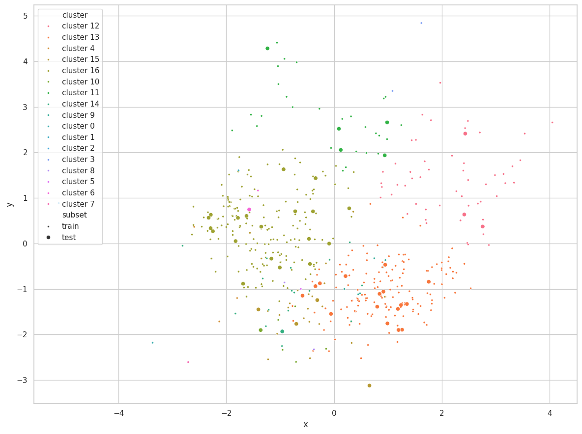
Discussions
We re-use the 99% energy reduction previously performed and select $e=5.0$, as higher values would create a massive central cluster and only two residual ones.
The results obtained here were very similar to the ones without the use of PCA. Once again, we observe clusters 0 and 1 containing a few sparsely positioned samples, while cluster 2 and 3 contain most samples of the set. Cluster 4 is positioned on the top-middle of the space, between 2 and 3, and contains fewer samples than both.
References
- H.-P. Kriegel, E. Schubert, and A. Zimek, “The (black) art of runtime evaluation: Are we comparing algorithms or implementations?,” Knowledge and Information Systems, vol. 52, no. 2, pp. 341–378, Aug. 2017,Available at: https://doi.org/10.1007/s10115-016-1004-2
- D. Arthur and S. Vassilvitskii, “k-means++: The advantages of careful seeding,” Stanford, 2006.
- T. Kurita, “Principal component analysis (PCA),” Computer vision: a reference guide, pp. 1–4, 2019.
- F. Murtagh and P. Contreras, “Algorithms for hierarchical clustering: an overview,” Wiley Interdisciplinary Reviews: Data Mining and Knowledge Discovery, vol. 2, no. 1, pp. 86–97, 2012.
- F. Pedregosa et al., “Scikit-learn: Machine Learning in Python,” Journal of Machine Learning Research, vol. 12, pp. 2825–2830, 2011.
- R. K. Pace and R. Barry, “Sparse spatial autoregressions,” Statistics & Probability Letters, vol. 33, no. 3, pp. 291–297, 1997.
- Wikipedia, “K-means clustering — Wikipedia, The Free Encyclopedia.” https://en.wikipedia.org/wiki/K-means_clustering, 2021.