The 2D Fourier Transform

Similarly to my previous post, I decided to publish here an assignment that was submitted to a Computer Vision class. Its goal is to apply the Discrete Fourier Transform over images using Python programming language and assess its results. Firstly, I implement low, high and band-pass circular filters in the frequency domain for 2D signals. Secondly, I present two examples: (a) a visualization of the frequency spectrum the when the original signal is rotated; and (b) an image compression strategy based on Fourier Transform.

TF-Flowers (Image Dataset)

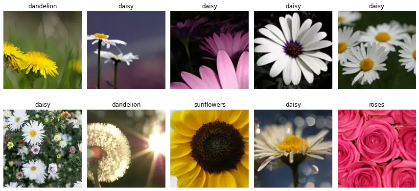
We utilize 10 random images from the TF-Flowers dataset, which can be downloaded in the tf-records format using the tensorflow-datasets library.

This dataset represents a multi-class (mono-label) image classification problem, and comprises 3,670 photographs of flowers associated with one of the following labels: dandelion, daisy, tulips, sunflowers or roses.

show setup code

import tensorflow as tf
import tensorflow_datasets as tfds


class Config:
    image_sizes = (300, 300)
    images_used = 10
    
    buffer_size = 8 * images_used
    seed = 68215

def preprocessing_fn(image, label):
  # Adjust the image to be at least of size `Config.image_sizes`, which
  # garantees the random_crop operation below will work.
  current = tf.cast(tf.shape(image)[:2], tf.float32)
  target = tf.convert_to_tensor(Config.image_sizes, tf.float32)
  ratio = tf.reduce_max(tf.math.ceil(target / current))
  new_sizes = tf.cast(current*ratio, tf.int32)

  image = tf.image.resize(image, new_sizes, preserve_aspect_ratio=True)
  image = tf.image.resize_with_crop_or_pad(image, *Config.image_sizes)

  return image, label

(train_ds,), info = tfds.load(
  'tf_flowers',
  split=['train[:1%]'],
  with_info=True,
  as_supervised=True)

int2str = info.features['label'].int2str

images_set = (train_ds
              .shuffle(Config.buffer_size, Config.seed)
              .map(preprocessing_fn, num_parallel_calls=tf.data.AUTOTUNE)
              .batch(Config.images_used)
              .take(1))

images, target = next(iter(images_set))
images = tf.cast(images, tf.float32)
labels = [int2str(l) for l in target]

Discrete Fourier Transform

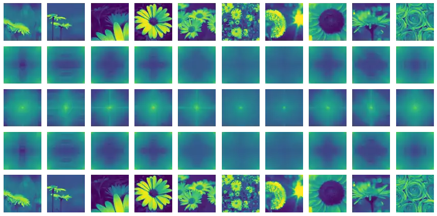
Identity

Proposed activity: apply the Fast Fourier Transform to an image and its inverse, detailing each step.

The application of the Fourier Transformation over images is straight forward: the function tf.signal.fft2d can be used to represent a tensor of shape $(b_0, b_1, \ldots b_n, h, w)$ in the frequency domain, where the two inner-most axes (namely, $h$ and $w$) are assumed to contain the information to be transformed and the remaining are assumed to be batch dimensions. The code below describes all steps involved in transforming a signal and reconstructing it its original domain.

x = tf.image.rgb_to_grayscale(images)

y = tf.cast(x, tf.complex64)
y = tf.signal.fft2d(y[..., 0])
s = tf.signal.fftshift(y, axes=(1, 2))
z = tf.signal.ifftshift(s, axes=(1, 2))
w = tf.signal.ifft2d(z)

Circular Low-pass Filter

Low-pass filters can be implemented as binary masks that retain low frequencies of a signal while suppressing high frequencies. A vectorized ideal circular filter can be implemented as described below. Two vectors are used in this implementation ($h$ and $w$). They represent the distance between each pixel and the signal center. The $h$ vector is reshaped into a column vector and the radius input vector is reshaped into $(r, 1, 1)$, where $r$ is the number of radii passed. Finally, the operation $h^2 + w^2 < \text{radius}^2$ will return a tensor of shape $(r, h, w)$, containing all filters built.

def as_absolute_length(measures, height, width):
  if isinstance(measures, (int, float)):
    measures = [measures]
  
  return tf.convert_to_tensor([
    (m
     if isinstance(m, int)
     else int(m*min(height, width) // 2))
    for m in measures
  ])


def circ_filter2d(radius, shape, dtype=tf.float32):
  if len(shape) == 4:
    h, w = shape[1:3]
  elif len(shape) == 3:
    h, w = shape[:2]

  ih = tf.abs(tf.range(h) -h//2)  # [... 2 1 0 1 2 ...]
  ih = tf.reshape(ih, (-1, 1))
  iw = tf.abs(tf.range(w) -w//2)

  radius = as_absolute_length(radius, h, w)
  radius = tf.reshape(radius, (-1, 1, 1))

  return tf.cast(ih**2 + iw**2 < radius**2, dtype)  # circle eq.

circ_filter2d_like = lambda radius, a: circ_filter2d(radius, a.shape, a.dtype)

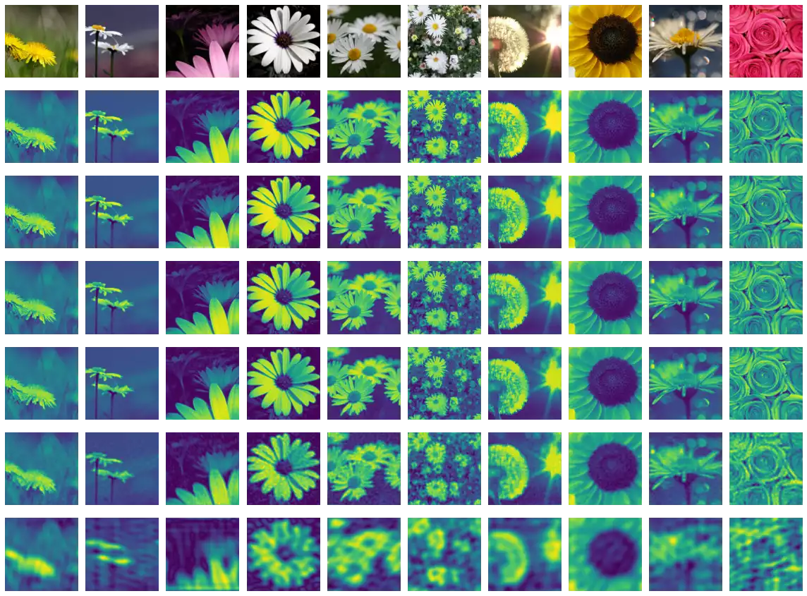
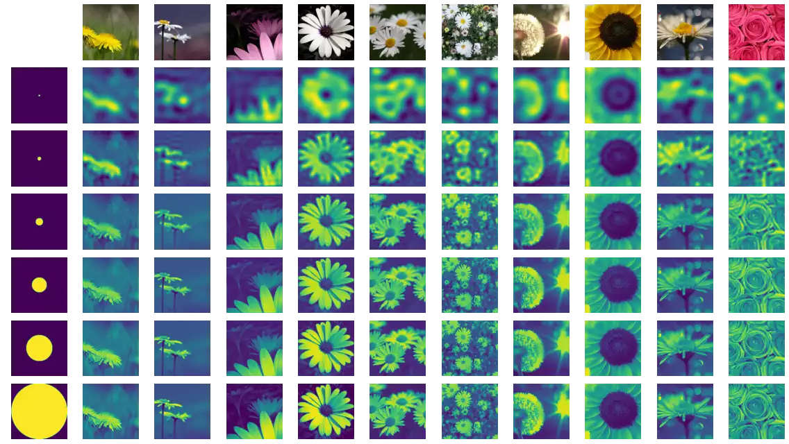
Figure 4 illustrates the steps in the low-pass filtering procedure of a signal in the frequency domain, while Figure 5 and Figure 6 illustrate the difference of the application of the ideal low-pass and Butterworth low-pass filters. A quality difference of the blur effect is clearly perceptible, where the Butterworth filter generates much better results for small radius arguments.

m = circ_filter2d_like(70, s[..., 0])
z = tf.signal.ifftshift(m * s[..., 0], axes=(1, 2))
w = tf.signal.ifft2d(z)

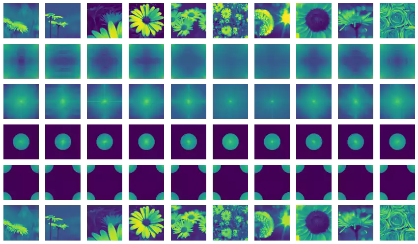
Experimenting with Multiple Radius Values

EXPERIMENTED_RADII = (5, 10, 20, 40, 70, 150)

masks = circ_filter2d_like(EXPERIMENTED_RADII, s)

m = masks[:, tf.newaxis, ...] * s
z = tf.signal.ifftshift(m, axes=(-2, -1))
w = tf.signal.ifft2d(z)

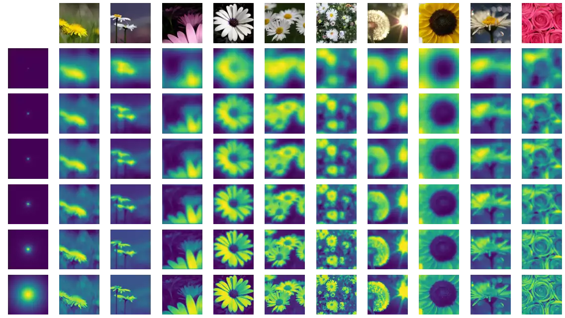
Butterworth Low-pass Filter

A Butterworth low-pass filter can be built similarly to the circular low-pass filter, by replacing the circle equation:

def butterworth_filter2d(radius, shape, n=1, dtype=tf.float32):
  h, w = shape[-2:]

  ih = tf.abs(tf.range(h) -h//2)
  ih = tf.reshape(ih, (-1, 1))
  iw = tf.abs(tf.range(w) -w//2)

  radius = as_absolute_length(radius, h, w)
  radius = tf.reshape(radius, (-1, 1, 1))

  return tf.cast(
    1 / (1 + (ih**2 + iw**2) / radius**(2*n)),
    dtype
  )

butterworth_filter2d_like = lambda radius, a, n=1: butterworth_filter2d(radius, a.shape, n, a.dtype)

EXPERIMENTED_RADII = (.01, .02, .03, .05, .1, .5)

masks = butterworth_filter2d_like(EXPERIMENTED_RADII, s)

m = masks[:, tf.newaxis, ...] * s
z = tf.signal.ifftshift(m, axes=(-2, -1))
w = tf.signal.ifft2d(z)

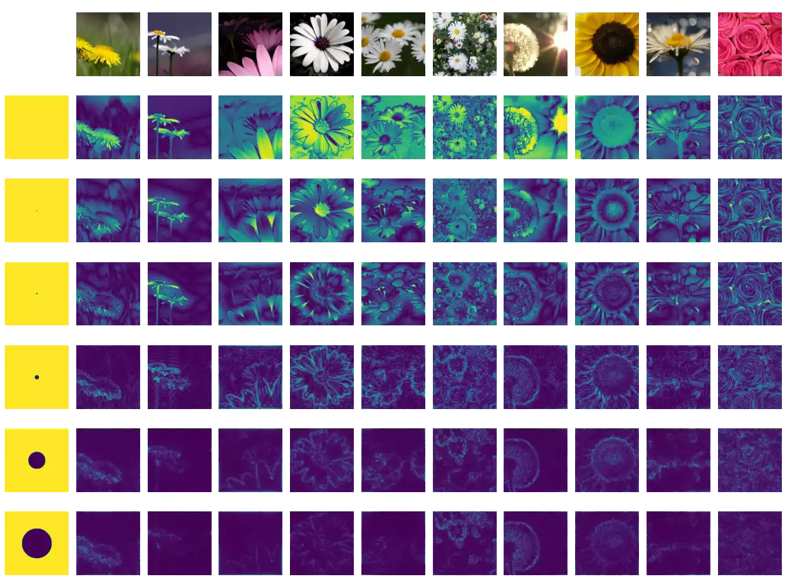
High-pass Filter

A ideal high-pass filter can be trivially obtained from the circ_filter2d function described above, by simply subtracting its result from 1. This will effectively switch every zero in the mask by one and vice versa. Figure 7 illustrates the application of multiple ideal high-pass filters over images. We notice textural information is removed and we are left with edge and boundary information of the original images.

EXPERIMENTED_RADII = (1, 2, 3, 10, 40, 70)

masks = 1 -circ_filter2d_like(EXPERIMENTED_RADII, s)

m = masks[:, tf.newaxis, ...] * s
z = tf.signal.ifftshift(m, axes=(-2, -1))
w = tf.signal.ifft2d(z)

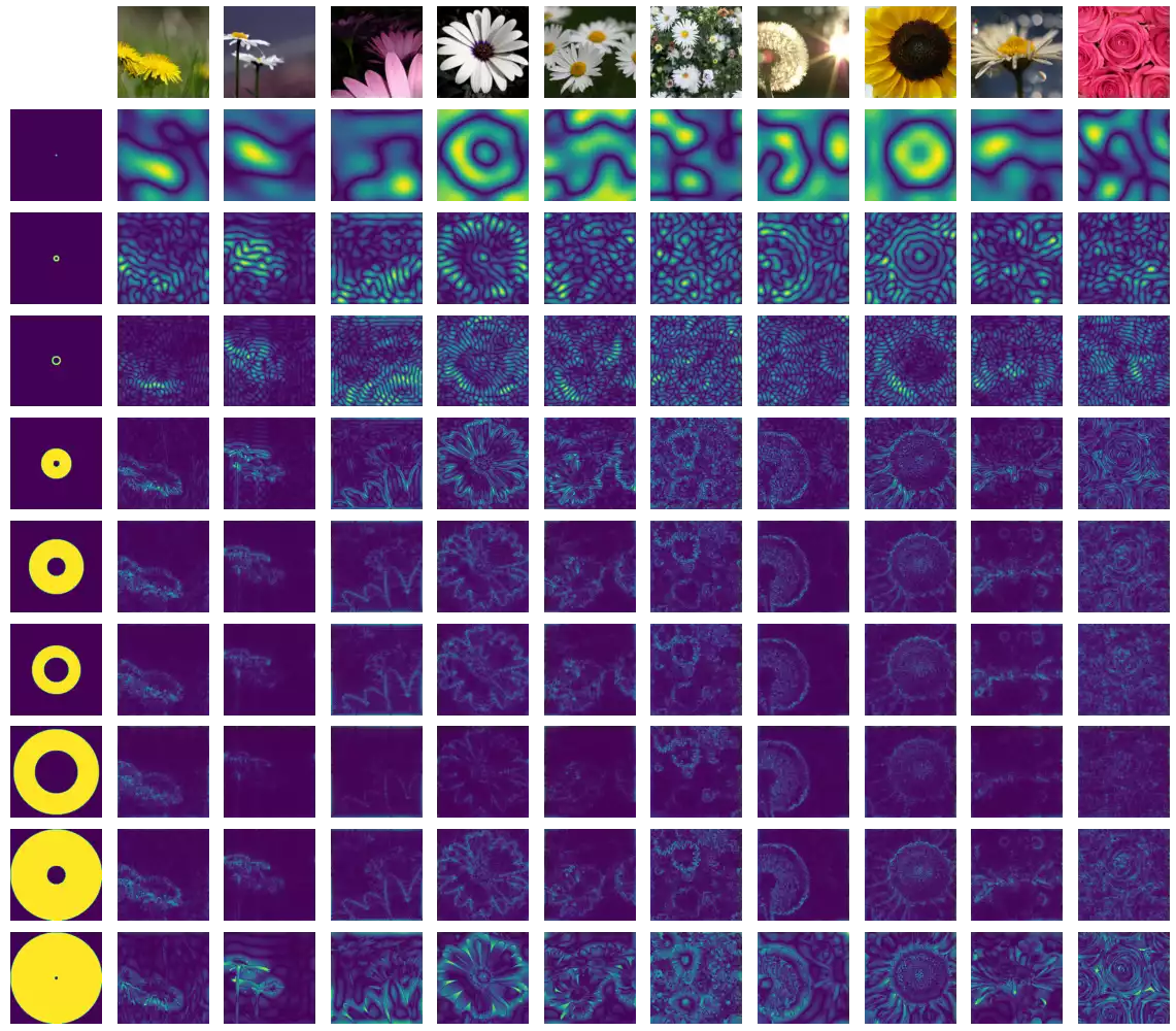
Band-pass Filter

I once again leverage the circ_filter2d function to create the ideal band-pass filter, consisting of the subtraction of two low-pass filters with different radii. Figure 8 illustrate the application of multiple ideal band-pass filters over images. Results are considerably harder to interpret, compared with the previous ones: filters with small inner radii and small width seem to capture very specific textural patterns; while filters with larger inner radii and large width seem to behave like high-pass filters.

RADII_L = (1, 5, 10, 10, 30, 40, 70, 30, 5)
RADII_H = (3, 10, 15, 50, 90, 80, 140, 150, 150)

masks = circ_filter2d_like(RADII_H, s) -circ_filter2d_like(RADII_L, s)

m = masks[:, tf.newaxis, ...] * s
z = tf.signal.ifftshift(m, axes=(-2, -1))
w = tf.signal.ifft2d(z)

Examples

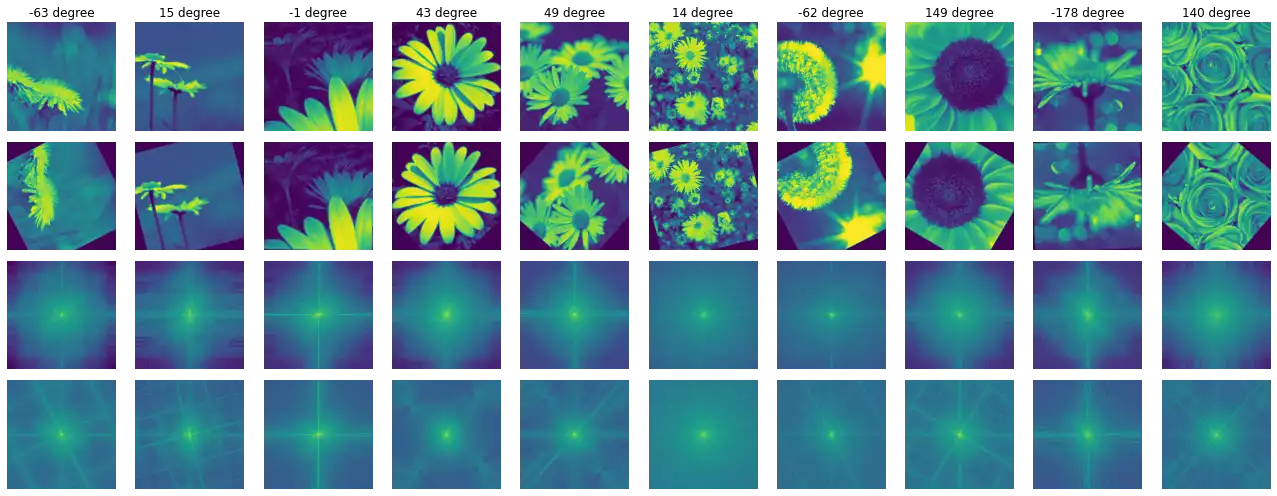
Spectrum Rotation

Figure 10 illustrates the effect observed in the spectrum of the signal generated by the DFT of a rotated input image. The spectrum is also rotated in the same angle as the input image.

import numpy as np
import tensorflow_addons as tfa

rotations = tf.random.normal(images.shape[:1]) * np.pi/2

r = tfa.image.rotate(x, rotations)

zx, zr = (tf.signal.fftshift(tf.signal.fft3d(tf.cast(z, tf.complex64)),
                             axes=(1, 2))
          for z in (x, r))

Compressing Images Using The DFT

Compression can be performed by nullifying coefficients, the magnitude of which does not reach a certain threshold. The code below describes a compression filter based on a percentile value for the magnitude. As TensorFlow does not provide statistical functions, we are forced to recur to the tensorflow_probability (tfp) library.

Figure 9 illustrates the compression of the images using multiple rates. I found the quality of images compressed with a rate below 95% to be very similar of the original copy, with visible quality deterioration being most noticeable at 99.9%.

import tensorflow_probability as tfp

THRESHOLDS = [10, 50, 90, 95, 99, 99.9]

masks = tf.abs(s)
th = tfp.stats.percentile(masks, THRESHOLDS, axis=(1, 2))
th = tf.transpose(th)
th = tf.reshape(th, (*th.shape, 1, 1))
masks = tf.cast(masks[:, tf.newaxis, ...] > th, tf.complex64)

m = masks * s[:, tf.newaxis, ...]
z = tf.signal.ifftshift(m, axes=(2, 3))
w = tf.signal.ifft2d(z)