A Vectorized Implementation of The Convolution Operation

In this post, I thought I shared an assignment I have recently done for a Computer Vision class.

Although results in Computer Vision are easily represented and interpreted, the implementation of even the most basic operations can be quite challenging. Even when the idea behind some code is trivial, implementations on GitHub and other websites can be quite difficult to understand. A few reasons come to mind, but I believe one to be of paramount importance: vectorization.

What’s Vectorization

The idea behind vectorization is to leverage the concurrency and cache mechanisms of modern processors (and clusters thereof) in order to more efficiently apply operations over an entire set of values, instead of sequentially executing these same operations over each value. For example, consider the basic add operation between two integers in Python:

a = 10
b = 20
c = a + b  # 30

In order to add a set of numbers, you must use a for loop:

a = [0, 1, 2, 3]
b = [5, 4, 3, 2]
c = [0, 0, 0, 0]

for i in range(len(a)):
  c[i] = a[i] + b[i]

As Python was created thinking in a broader context than scientific and numerical applications, not all operators behave exactly as we have seen in linear algebra and calculus classes. For example, adding two lists in python results in the concatenation of these two lists: [0, 1, 2] + [4, 3, 2] = [0, 1, 2, 4, 3, 2]. Additionally, all lists in Python are implemented as doubly linked rings, in which the last element is doubly linked to the first element. Although this structure guarantees best insertion and deletion times, it does not guarantee data contiguous allocation in memory, thus not optimizing cache hit.

Libraries such as NumPy, SciPy and TensorFlow play a important role in cPython vectorization. Being mostly written in the C and C++ programming language (while exposing a Python interface), they allow us to work with memory-contiguous arrays, and overwrite most numeric operators to match their counterparts’ behavior in scientific and numeric applications.

Using numpy, you can transparently add two arrays using vectorization:

a = np.asarray([0, 1, 2, 3])
b = np.asarray([5, 4, 3, 2])
c = a + b  # == (5, 5, 5, 5)

Of course, everything else also works:

c = a + b  # pair-wise sum                   == (5, 5, 5, 5)
c = a - b  # pair-wise sub                   == (-5, -3, -1, 1)
c = a * b  # pair-wise mul                   == (0, 4, 6, 6)
c = a / b  # pair-wise div                   == (0, 1/4, 2/3, 3/2)
c = a % b  # pair-wise mod                   == (0, 1, 2, 1)
c = a @ b  # matrix mul (inner product here) == 16
c = 2 * a  # scalar mul                      == (0, 2, 4, 6)
c = a**2   # element-wise power              == (0, 1, 4, 9)

Other interesting examples:

c = a.reshape((2, 2))  # reshaping vector into matrix == ((0, 1)
                       #                                  (2, 3))
d = c.T                # transposing                  == ((0, 2),
                       #                                  (1, 3))
e = c @ d              # matrix mul                   == ((1, 3),
                       #                                  (3, 13))
e = e.ravel()          # re-linearizing matrix        == (1, 3, 3, 13)

f = np.random.randn(3, 2, 2)  # random normal numbers  == (((n0, n1), (n2, n3)),
                              #                            ((n4, n5), (n6, n7))
                              #                            ((n8, n9), (n10, n11)))
g = f + c                     # broad-cast sum         == (((n0+0, n1+1), (n2+2, n3+3)),
                              #                            ((n4+0, n5+1), (n6+2, n7+3))
                              #                            ((n8+0, n9+1), (n10+2, n11+3)))

As Machine Learning is full of linear algebra, we can efficiently represent pretty much any operation with vectorization:

x = np.random.randn(32, 64)
w = np.random.randn(64, 10)
b = np.zeros(10)

x @ w + b         # dense layer of a NN, followed by ReLU activation
np.maximum(, 0)   # ReLU activation function
e**x / (1-e**-x)  # Sigmoid activation function

x -= x.mean(axis=1)  # Data standardization
x /= x.std(axis=1)   #

x -= x.min(axis=1)   # Data normalization
x /= x.max(axis=1)   #

TF-Flowers (Image Dataset)

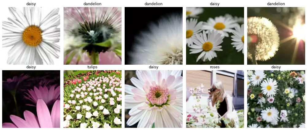
In order to demonstrate the results, I utilized 10 random images from the TF-Flowers dataset, which can be downloaded in the tf-records format using the tensorflow-datasets library.

This dataset represents a multi-class (mono-label) image classification problem, and comprises 3,670 photographs of flowers associated with one of the following labels: dandelion, daisy, tulips, sunflowers or roses.

During the loading procedure, 1% of the set is retrieved from the disk (approximately 37 samples). Samples are shuffled and the first batch of 10 images is retrieved. In these settings:

• 3,670 images are downloaded into disk (compressed tf-record format)
• 37 (approx.) references — consisting of filepaths and record shard-level address — are loaded into memory
• 10 samples and labels are effectively loaded into memory

Images are represented by tensors of rank 3, of shape (HEIGHT, WIDTH, 3). They are first loaded into memory as n-dimensional arrays of type tf.uint8. As many of the following operations are floating point precision, we opted to cast them imediately to tf.float32. This is the default dtype for most operations in TensorFlow graphs.

Image may have different sizes, which prevents them from being directly stacked into a 4-rank tensor (BATCH, HEIGHT, WIDTH, 3). We circumvented this problem using the following procedure:

1. Let $Q := (300, 300, 3)$ be a desired output shape and $S_I := (H, W, 3)$ be the actual shape of any given image $I$.
   $I$ is resized so it’s smallest component (width or height) would match the smallest component of $Q$ (namely, 300), resulting in $I’$.

2. The largest component in the shape of $I’$ is now greater or equal to $300$. We extract the central crop of size $(300, 300)$ from $I’$, resulting inadvertly in an image of shape $(300, 300, 3)$.

show setup code

from math import ceil

import numpy as np
import tensorflow as tf
import tensorflow_datasets as tfds


class Config:
    image_sizes = (300, 300)
    images_used = 10

    buffer_size = 8 * images_used
    seed = 6714

def preprocessing_fn(image, label):
  # Adjust the image to be at least of size `Config.image_sizes`, which
  # garantees the random_crop operation below will work.
  current = tf.cast(tf.shape(image)[:2], tf.float32)
  target = tf.convert_to_tensor(Config.image_sizes, tf.float32)
  ratio = tf.reduce_max(tf.math.ceil(target / current))
  new_sizes = tf.cast(current*ratio, tf.int32)

  image = tf.image.resize(image, new_sizes, preserve_aspect_ratio=True)

  # Crop randomly.
  image = tf.image.resize_with_crop_or_pad(image, *Config.image_sizes)

  return image, label

(train_ds,), info = tfds.load(
  'tf_flowers',
  split=['train[:1%]'],
  with_info=True,
  as_supervised=True)

int2str = info.features['label'].int2str

images_set = (train_ds
              .shuffle(Config.buffer_size, Config.seed)
              .map(preprocessing_fn, num_parallel_calls=tf.data.AUTOTUNE)
              .batch(Config.images_used)
              .take(1))

images, target = next(iter(images_set))
images = tf.cast(images, tf.float32)
labels = [int2str(l) for l in target]

visualize(tf.cast(images, tf.uint8), labels)

Challenges

The following sections describe different challenges involving applying vectorized operations over images.

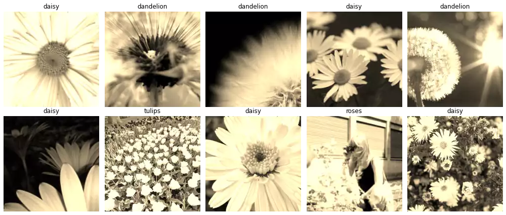
Challenge: Apply the sepia filter to a batch of images.

R = 0.393R + 0.769G + 0.189B
G = 0.349R + 0.686G + 0.168B
B = 0.272R + 0.534G + 0.131B

One way to perform this is to separate the image tensor $I$ of shape (B, H, W, 3) by its last axis, forming three tensors of shape (B, H, W, 1). We multiply each and every component according to the rule above and concatenate the result:

@tf.function
def sepia(x):
  x = tf.cast(x, tf.float32)

  r, g, b = tf.split(x, 3, axis=-1)

  y = tf.concat((0.393*r + 0.769*g + 0.189*b,
                 0.349*r + 0.686*g + 0.168*b,
                 0.272*r + 0.534*g + 0.131*b),
                axis=-1)

  return tf.clip_by_value(y, 0, 255)

A more ellegant solution is to remember that every linear system (including $(R’, G’, B’)^\intercal$, described above) can be interpreted as a multiplication between the input matrix and a coefficient matrix:

In our case, $I$ has rank 4 (not a matrix), but the same equivalence applies, as the matrix multiplication is a specific case of the tensor dot product. There are multiple ways to perform this operation in TensorFlow:

1. y = tf.matmul(x, s): inner-product over the inner-most indices in the input tensors (last axis of x and antepenultimate axis of s). This assumes the other axes represent batch-like information, and generalizes the matrix-multiplication operation for all cases (the input is a matrix, batch of matrix or batch of sequence of matrix, …).

2. y = x @ s: override of tf.matmul, same resulting operation

3. y = tf.tensorproduct(x, s, 1): the tensor dot product over one rank (the last in x and first in sepia_weights):

4. y = tf.einsum('bhwc,ck->bhwk', x, s): Einstein’s summation over the rank c (last in x and first in s)

sepia_weights = tf.constant(
  [[0.393, 0.349, 0.272],
   [0.769, 0.686, 0.534],
   [0.189, 0.168, 0.131]]
)

@tf.function
def sepia(x):
  y = x @ sepia_weights
  return tf.clip_by_value(y, 0, 255)


images_s = sepia(images)

show code

visualize(
  tf.cast(images_s, tf.uint8),
  labels
)

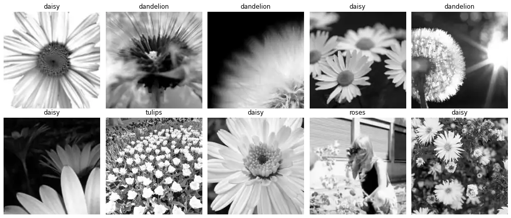
Challenge: Transform a batch of RGB images into gray-scale images.

I = 0.2989R + 0.5870G + 0.1140B

The solution is very similar to what was done above, except that the coefficient tensor is no longer a matrix, which preclude the usage of @. We use tf.tensordot to compute the inner product between the last axis of x and first (and only) axis of gray_weights.

An acceptable alternative form would be tf.einsum('bhwc,c->bhw', x, gray_weights).

gray_weights = tf.constant([0.2989, 0.5870, 0.1140])

@tf.function
def grayscale(x):
  y = tf.tensordot(x, gray_weights, 1)
  y = tf.expand_dims(y, -1)             # restore 3rd rank (H, W, 1)
  return tf.clip_by_value(y, 0, 255)

images_g = grayscale(images)

show code

visualize(
  tf.cast(images_g, tf.uint8),
  labels,
  cmap='gray'
)

Challenge: Apply the following filters to the monochromatic images.

show kernels

h17 = tf.constant(
  [
    [[-1., 0., 1.],
     [-2., 0., 2.],
     [-1., 0., 1.]],

    [[-1., -2., -1.],
     [ 0.,  0.,  0.],
     [ 1.,  2.,  1.]],

    [[-1., -1., -1.],
     [-1.,  8., -1.],
     [-1., -1., -1.]],
   
    [[1/9, 1/9, 1/9],
     [1/9, 1/9, 1/9],
     [1/9, 1/9, 1/9]],

    [[-1., -1.,  2.],
     [-1.,  2., -1.],
     [ 2., -1., -1.]],

    [[ 2., -1., -1.],
     [-1.,  2., -1.],
     [-1., -1.,  2.]],

    [[ 0., 0., 1.],
     [ 0., 0., 0.],
     [-1., 0., 0.]],
  ]
)

h8 = tf.constant(
  [[ 0.,  0., -1.,  0.,  0.],
   [ 0., -1., -2., -1.,  0.],
   [-1., -2., 16., -2., -1.],
   [ 0., -1., -2., -1.,  0.],
   [ 0.,  0., -1.,  0.,  0.]]
)

h9 = 1/256 * tf.constant(
  [[1.,  4.,  6.,  4., 1.],
   [4., 16., 24., 16., 4.],
   [6., 24., 36., 24., 6.],
   [4., 16., 24., 16., 4.],
   [1.,  4., 16.,  4., 1.]]
)

h89 = tf.stack((h8, h9), axis=0)

h17 = tf.transpose(h17, (1, 2, 0))
h89 = tf.transpose(h89, (1, 2, 0))

Convolution Basics

The convolution of a 1-D input sinal $f$ and a 1-D kernel $g$ is defined as the integration of the product between the two signals, when evaluated over the temporal component:

We observe from the equation above that one of the signals is reflected. This is essential so both functions are evaluated over the same time interval, resulting in the effect of “zipping” the two functions together. This effect is illustrated in the first column of the figure below.

On the other hand, Cross-correlation is a similar operation in which $g$ slides over $f$ without the aforementioned reflection:

The signals are associated in an inverted fashion, which is illustrated in the second column of the figure below.

Finally, we can imagine that a 2-D signal (such as images) is reflected when both $(x, y)$ axes are reflected. This is equivalent of rotating the image in $180^\circ$.

Using TensorFlow’s Native Conv2D Implementation

Notwithstanding its name, the tf.nn.conv2d(f, g) function implements the cross-correlation function, and the convolution operation is supposedly performed by assuming the kernel $g$ is already reflected.

In the example below, we observe the output signal is obtained by the Cross-correlation eq.:

s = tf.constant(
  [[1., 2., 3.],
   [4., 5., 6.],
   [7., 8., 9.]]
)
k = tf.constant(
  [[1., 1.],
   [0., 0.]]
)
c = tf.nn.conv2d(
  tf.reshape(s, (1, 3, 3, 1)),
  tf.reshape(k, (2, 2, 1, 1)),
  strides=1,
  padding='VALID'
)

print('signal:', s.numpy(), sep='\n')
print('kernel:', k.numpy(), sep='\n')
print('s*k:', tf.reshape(c, (2, 2)).numpy(), sep='\n')

signal:
[[1. 2. 3.]
  [4. 5. 6.]
  [7. 8. 9.]]
kernel:
[[1. 1.]
  [0. 0.]]
s*k:
[[ 3.  5.]
  [ 9. 11.]]

This is a design decision which takes performance into account, as the rotation operations can be omitted during the feed-forward process. During training, kernels are correctly learnt through back-propagation by minimizing a given loss function (e.g. cross-entropy, N-pairs, focal loss). Interestingly enough, the differential of the real-valued cross-correlation with respect to its kernel (which is used to update the kernels) is the cross-correlation itself, rotated $180^\circ$ (e.g. convolution).

In this case, in which the kernels are fixed, we assume they represent regular filters. We therefore rotate the kernels them before applying the tf.nn.conv2d function.

This assignment can be trivially solved using this function:

def to_kernel(k):
  if len(k.shape) == 2: k = k[..., tf.newaxis]
  if len(k.shape) == 3: k = k[..., tf.newaxis, :]
  
  k = tf.image.rot90(k, 2)

  return k

y17 = tf.nn.conv2d(images_g, to_kernel(h17), 1, 'SAME')
y89 = tf.nn.conv2d(images_g, to_kernel(h89), 1, 'SAME')

yr1c2 = tf.sqrt(
  tf.nn.conv2d(images_g, to_kernel(h17[..., 0]), 1, 'SAME')**2 +
  tf.nn.conv2d(images_g, to_kernel(h17[..., 1]), 1, 'SAME')**2
)

y = tf.concat((y17, y89, yr1c2), axis=-1)
y = tf.clip_by_value(y, 0, 255)

Vectorized Cross-correlation Implementation

In this subsection, I present my implementation (and derivation thereof) of the 2-dimensional convolution function. For simplicity, it is implemented as the correlation between an input signal $s$ and the reflection of an input kernel $k$.

Study of a Use Case

I decided to start by considering a simple use case. For analytical convenience, I imagined this case to have the following characteristics:

• Only one image $s$ and one kernel $k$ are involved in this operation.
• No padding is performed in the input signal (i.e. padding valid).
• $s$ and $k$ have different height and width values — namely, $(H_s, W_s)$ and $(H_k, W_k)$ —, and they are prime numbers. This is interesting when flattening a matrix into a vector, as prime numbers have distinct products and will result in dimensions that are easier to understand.
• The kernel is not symmetric. Hence the convolution and cross-correlation functions will result in different signals.

I considered the following signals in my use-case:

show code

s = np.arange(35).reshape((7, 5))
k = np.asarray([[0, 2, 1],
                [0, 1, 0]])

I simulated the effect of a 2-D kernel $k$ sliding across the spatial dimensions of $s$ by “extracting” multiple non-mutually disjointed subsections of the image into a sequence of flattened patches, which could then be broadcast-multiplied by the flattened kernel and reduced with the sum operation. To make this “extraction” more efficient, an index-based mask was built and applied over the image. This approach requires the construction of two integer matrices $R$ and $C$ — each of shape $((H_s-H_k+1)(W_s-W_k+1), H_k W_s)$ —, but does not replicate the values contained within the input signal $s$. Rather, index-based masks create merely views of the n-dimensional arrays over which they are applied.

The indexing procedure can be described by the following steps.

• The window starts at the first valid position in matrix $s$, and references the sub-matrix $s[0:2,0:2]$ with the flatten index vector $[(0,0), (0,1), (0,2), (1,0), (1,1),(1,2)]$ or, for briefness, $\begin{bmatrix}00 & 01 & 02 & 10 & 11 & 12\end{bmatrix}$.
• $k$ slides horizontally until the last valid index of $s$, yielding $W_s-W_k+1$ index vectors in total.
• The window resets at the column of $s$, but positioned at the next following row.
• The three steps above are repeated for each valid vertical index ($H_s-H_k+1$ times), effectively covering all sections of the matrix $s$.

The use-case represented above can therefore be indexed as:

We can identify multiple patterns in the matrix above.

Firstly, onto the vertical indexing (i.e., the index $r$ in the index pair $rc$, for $M_s = [rc]_{R\times C})$. In the first column, $r$ is arranged from $0$ to $H_s-H_k+1$, and each number repeats $W_s-W_k+1$ times. This can be expressed in numpy notation as:

B, H, W = s.shape
KH, KW, KC = k.shape

r0 = np.arange(H-KH+1)
r0 = np.repeat(r0, W-KW+1)
r0 = r0.reshape(-1, 1)

Across the rows, $r$ repeats itself $W_k$ times, and then it assumes the value $r+1$ and repeats itself $W_k$ times once again. These two outer-most repetitions are due to the fact that the kernel has 2 rows. In a general case, we would observe $H_k$ repetitions:

r1 = np.arange(KH).reshape(1, KH)
r = np.repeat(r0 + r1, KW, axis=1)

Notice that the addition between a column vector $r_0$ and a row vector $r_1$ will construct a matrix through broadcasting. The matrix $R$ now contains the first index in $M_s$.

As for the horizontal indexing $c$, we observe the numbers are sequentially arranged in the first row from 0 to $W_k$, and that this sequence repeats $H_k$ times:

c0 = np.arange(KW)
c0 = np.tile(c0, KH).reshape(1, -1)

Furthermore, $c$ increases by 1 each row (as our convolution slides by exactly 1 step), going up to the number of horizontal slide steps of $k$ onto $s$ ($W_s-W_k+1$). Adding this row vector to $c_0$ (a column vector) produces the index matrix for all horizontal slides of the kernel. Finally, we vertically tile (outer repeat) this matrix by the number of valid horizontal slide steps ($H_s-H_k + 1$):

c1 = np.arange(W-KW+1).reshape(-1, 1)
c = np.tile(c0 + c1, [H-KH+1, 1])

Hence, $M_s = [R, C]$.

Additional Considerations

Batching

As $M_s$ was constructed taking the width and height of the signals into consideration, it does not depend on the number of images, nor the number of kernels. Let $s$ be redefined as a signal of shape $(B_1, B_2, \ldots, B_n, H_s, W_s)$ (a batch of batches of \ldots batches of images), and $k$ a signal of shape $(H_k, W_k, C)$ This solution can be easily extended to a multi-image, multi-kernel scenario by broadcasting the index-mask selection of $s$ to all batch-like dimensions and dotting it with the flatten kernels:

y = s[..., r, c] @ k.reshape(-1, C)

Padding

As kernels of sizes greater than 0 slide across the spatial dimensions of an input signal $s$, they will occupy at most $(H_s-H_k+1)\times (W_s-W_k+1) < H_s W_s$ positions, resulting in an output signal smaller than the input signal. More specifically, of shape $(B_1, B_2, \ldots, B_n, H_s-H_k+1, W_s-W_k+1, C)$. One can imagine many cases in which the maintenance of the signal size is desirable, such as maintaining locality between multiple applications of the convolution; or maintaining visualization consistency.

In order to maintain a consistent signal shape, I implemented the flag padding='SAME', what is sometimes referred to as zero-padding. I employed here a strategy similar to what is done in the NumPy and TensorFlow libraries: $(H_k-1, W_k-1)$ zeros are added to the input signal’s height and width respectively. During the convolution, the spatial dimensions of the input signal become $((H_s+H_k-1)-H_k+1, (W_s+W_k-1)-W_k+1) = (H_s, W_s)$.

For kernels with an odd numbered width and height, this operation becomes trivial: we add $\lfloor H_k/2 \rfloor$ rows to both top and bottom extremities of the signal, and $\lfloor W_k/2 \rfloor$ columns to its left and right extremities.

A particular case must be handled when one of the sizes of the kernel is even: adding $\lfloor H_k/2 \rfloor$ will result in an output signal larger than the input signal by exactly 1 pixel. I handled this case in the same manner NumPy seemly does, by adding more padding to the bottom/right than to the top/left.

Usage Conditions and Limitations

The input signal (images) must be in the shape of $(B_1, B_2, \ldots, B_n, H_s, W_s)$ and kernels must be in the shape of $(H_k, W_k, C)$. I also remark the following important limitations of this implementation:

• This function is limited to the two dimensional spatial case, and will not work correctly for 3-D, 4-D and, more generally, n-D spatial signals, where $n > 3$.
• Stride is always 1, which makes this function unsuitable for Atrous Convolution.

Complete Implementation

from math import ceil, floor

_PADDINGS = ('VALID', 'SAME')

def _validate_correlate2d_args(s, k, padding):
  assert padding in _PADDINGS, (f'Unknown value {padding} for argument `padding`. '
                                f'It must be one of the following: {_PADDINGS}')
  assert len(s.shape) == 3, (f'Input `s` must have shape [B, H, W]. '
                             f'A tensor of shape {s.shape} was passed.')
  assert len(k.shape) == 3, (f'Kernels `k` must have shape [H, W, C]. '
                             f'A tensor of shape {k.shape} was passed.')


def correlate2d(s, k, padding='VALID'):
  s, k = map(np.asarray, (s, k))
  _validate_correlate2d_args(s, k, padding)

  B, H, W = s.shape
  KH, KW, KC = k.shape

  if padding == 'SAME':
    pt, pb = floor((KH-1)/2), ceil((KH-1)/2)
    pl, pr = floor((KW-1)/2), ceil((KW-1)/2)

    s = np.pad(s, ((0,0), (pt, pb), (pl, pr)))
    B, H, W = s.shape
  
  # Creating selection tile s[0:3, 0:3]
  #   --> [s[0,0], s[0,1], s[0,2], s[1,0], s[1,1], s[1,2]]
  r0 = np.arange(H-KH+1)
  r0 = np.repeat(r0, W-KW+1)
  r0 = r0.reshape(-1, 1)

  r1 = np.arange(KH).reshape(1, KH)
  r = np.repeat(r0 + r1, KW, axis=1)

  c0 = np.arange(KW)
  c0 = np.tile(c0, KH).reshape(1, -1)

  c1 = np.arange(W-KW+1).reshape(-1, 1)
  c = c0 + c1
  c = np.tile(c, [H-KH+1, 1])

  # k.shape (3, 3) --> (9, 1), in order to multiply
  # and add-reduce in a single pass with "@".
  y = s[..., r, c] @ k.reshape(-1, KC)
  y = y.reshape(B, H-KH+1, W-KW+1, KC)

  return y

def convolve2d(s, k, padding='VALID'):
  k = np.rot90(k, k=2)  # reflect signal.
  return correlate2d(s, k, padding)

Testing My Implementation Against Scipy’s

One way of testing this code is to compare the results with scipy’s implementation. We can use the np.testing.assert_almost_equal function to compare arrays (up to the 6th decimal), which will either pass without errors or print how similar the two arrays are:

import scipy.signal

for padding in ('valid', 'same'):
  y_mine = correlate2d(s, k, padding=padding.upper())
  y_scipy = np.asarray(
    [
      [scipy.signal.correlate2d(s[b], k[..., c], mode=padding.lower())
       for c in range(k.shape[-1])]
      for b in range(s.shape[0])
    ]
  ).transpose(0, 2, 3, 1)  # transpose to (B, H, W, C) format.

  np.testing.assert_almost_equal(
    y_mine,
    y_scipy
  )

print('All tests passed (no exceptions raised).')

All tests passed (no exceptions raised).

Application over TF-Flowers Image Samples

show code

y = np.concatenate(
  (convolve2d(images_g[..., 0].numpy(), h17, padding='SAME'),
   convolve2d(images_g[..., 0].numpy(), h89, padding='SAME')),
  axis=-1
)

yr1c1 = np.sqrt(
  convolve2d(images_g[..., 0].numpy(), h17[..., 0:1], padding='SAME')**2
  + convolve2d(images_g[..., 0].numpy(), h17[..., 1:2], padding='SAME')**2
)

y = np.concatenate((y, yr1c2), axis=-1)

visualizing = tf.cast(
  tf.clip_by_value(
    tf.reshape(
      tf.transpose(tf.concat((images_g, y), axis=-1), (0, 3, 1, 2)),
      (-1, *images_g.shape[1:])
    ),
    0,
    255
  ),
  tf.uint8
).numpy()

visualizing = [
  None,  # empty cell (original images column)
  *tf.transpose(h17, (2, 0, 1)).numpy(),  # kernels 1 through 7
  *tf.transpose(h89, (2, 0, 1)).numpy(),  # kernels 8 and 9
  None,  # empty cell (sqrt(s*h1^2+s^h2^2) column)
  *visualizing # images and convolution results
]

titles = [
  'original',
  *(f'$s*h_{i+1}$' for i in range(9)),
  '$\sqrt{ {s*h_1}^2 + {s*h_2}^2}$',
]

visualize(
  visualizing,
  titles,
  rows=images_g.shape[0] + 1,
  cols=y.shape[-1] + 1,
  figsize=(24, 25),
)

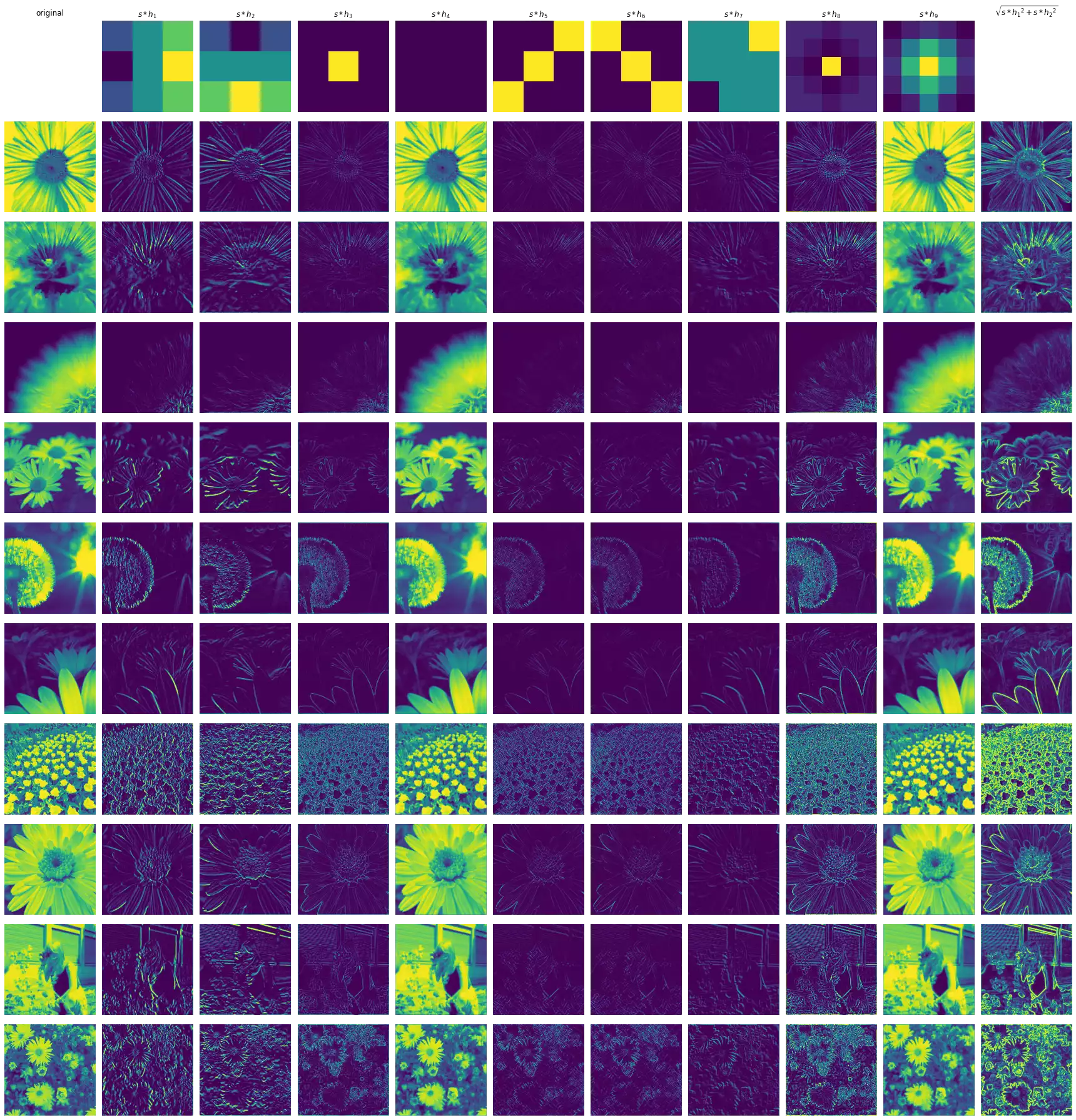
The figure above illustrates the result of the convolution of multiple input images with each kernel. A brief description of each result is provided below.

• H1 highlights regions containing vertical lines, in which the left side represents areas with higher activation intensity, while the ones in the right are dark regions.
• H2 is similar to H1, but activates strongly over horizontal lines in which the top is brighter than the bottom.
• H3 responds strongly to bright regions that are surrounded by dark regions in the input. It seems to extract fine edges regardless of their orientation.
• H4 is the uniform blur filter. It runs across the image macro-averaging the pixel activation intensities, reducing their differences.
• H5 detects diagonal (bottom-left to top-right) lines — this kernel is symmetric, hence the convolution results in the same signal as the correlation.
• H6 similar to H5, but detects diagonal (top-left to bottom-right) lines.
• H7 responds to regions with bright top-right corners and dark bottom-right corners, without taking into consideration the information in the in-between section (most of which is multiplied by 0).
• H8 is an edge-detector like H3, but seemly results in more detailed edges for these highly-detailed input images.
• H9 is the Gaussian blur filter. It weight-averages the differences between the intensities of the pixels giving the central region more importance.
• H10 combines H1 and H2 into one signal that seems to respond to both vertical and horizontal lines in the same intensity.