
Following the pattern of my previous posts, this one is based on an assignment submitted to the class of 2021/1 of course Introduction to Image Processing (MO443) at Universidade Estadual de Campinas. Its goal is to apply segmentation algorithms over images and extract characteristics of the objects using Python programming language and assess its results.
from math import ceil
from functools import partial as ftpartial

import numpy as np
import pandas as pd

import matplotlib.pyplot as plt

import os
import skimage.io
import skimage.filters
import skimage.feature
import skimage.segmentation

from skimage.color import label2rgb

import seaborn as sns

sns.set()

C = sns.color_palette("Set3")

def partial(func, *args, **kwargs):
    partial_func = ftpartial(func, *args, **kwargs)
    partial_func.__name__ = (f"{func.__name__} {' '.join(map(str, args))}"
                             f" {' '.join((f'{a}={b}' for a, b in kwargs.items()))}")
    return partial_func

def visualize(
    image,
    title=None,
    rows=2,
    cols=None,
    cmap=None,
    figsize=(12, 6)
):
    if image is not None:
        if isinstance(image, list) or len(image.shape) > 3:  # many images
            fig = plt.figure(figsize=figsize)
            cols = cols or ceil(len(image) / rows)
            for ix in range(len(image)):
                plt.subplot(rows, cols, ix+1)
                visualize(image[ix],
                          cmap=cmap,
                          title=title[ix] if title is not None and len(title) > ix else None)
            plt.tight_layout()
            return fig

        if image.shape[-1] == 1: image = image[..., 0]
        plt.imshow(image, cmap=cmap)

    if title is not None: plt.title(title)
    plt.axis('off')

def plot_segments(g, s, p, alpha=0.8, ax=None, linewidth=1):
    ax = ax or plt.gca()
    ax.imshow(label2rgb(s, image=g, bg_label=0, alpha=alpha, colors=C, bg_color=(1,1,1)))
    ax.axis('off')

    for i, region in p.iterrows():
        minr, minc, maxr, maxc = region['bbox-0'], region['bbox-1'], region['bbox-2'],region['bbox-3']
        rect = plt.Rectangle((minc, minr), maxc - minc, maxr - minr, fill=False,
                             edgecolor=C[i % len(C)], linewidth=linewidth)
        ax.add_patch(rect)

        plt.text(region['centroid-1'], region['centroid-0'], int(region.label))

def plot_detection_boxes(p, ax=None, linewidth=1):
    if ax is None:
        ax = plt.gca()

    H, W, C = p['image'].shape
    bboxes = p['objects']['bbox'].numpy()
    labels = p['objects']['label'].numpy()

    for b, l in zip(bboxes, labels):
        minr, minc, maxr, maxc = b
        minr, minc, maxr, maxc = minr*H, minc*W, maxr*H, maxc*W
        rect = plt.Rectangle((minc, minr), maxc - minc, maxr - minr, fill=False,
                             edgecolor=C[l % len(C)], linewidth=linewidth)
        ax.add_patch(rect)
        ax.text(minc,minr, int2str(l))
Segmentation and Detection of Simple Geometric Shapes
Using scikit-image, multiple segmentation strategies are available. For instance, one can extract borders [1] and label the connected regions; or find central regions and apply label expansion methods such as Watershed [2].
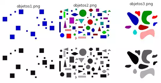
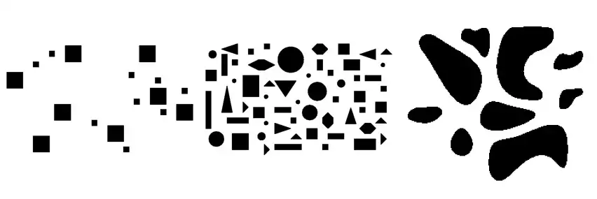
In the following sections, we exemplify two strategies (edge-based segmentation and the Felzenszwalb’s method) over simple geometric shapes, illustrated in the figure below.
image_files = sorted(os.listdir(Config.data.path))
images = [skimage.io.imread(os.path.join(Config.data.path, f)) for f in image_files]
grays = [skimage.color.rgb2gray(i) for i in images]

visualize([*images, *grays], image_files, cmap='gray');
Edge-Based Segmentation
Scikit-image implements many of the border extraction methods available in the literature, such as Sobel, Prewitt and Scharr [1]. The can be trivially used as described below.
%%time

N = 3

methods = [
  skimage.filters.sobel,
  skimage.filters.roberts,
  skimage.filters.prewitt,
  skimage.filters.farid,
  skimage.filters.scharr,
  partial(skimage.feature.canny, sigma=0.),
  partial(skimage.feature.canny, sigma=0.1),
  partial(skimage.feature.canny, sigma=3.),
]

segments = [[m(g) for g in grays] for m in methods]
CPU times: user 381 ms, sys: 4.75 ms, total: 386 ms
Wall time: 389 ms
method_names = [n.__name__ for n in methods]

visualize(grays, image_files, rows=1, cmap='gray');

for n, s in zip(method_names, segments):
  visualize(s, [n], rows=1, cmap='gray_r');
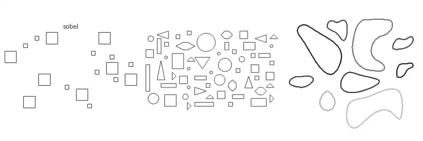
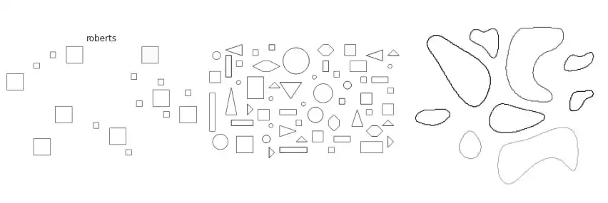
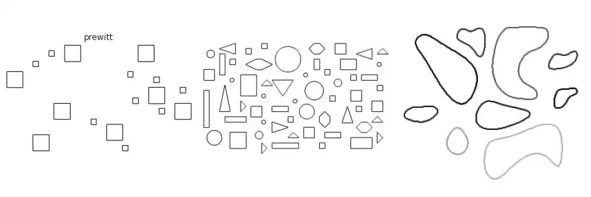
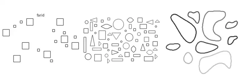
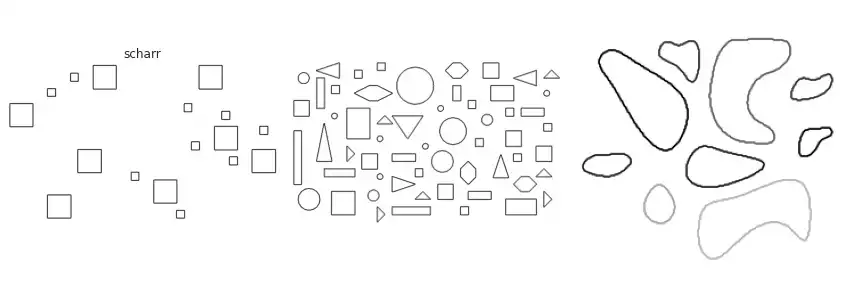
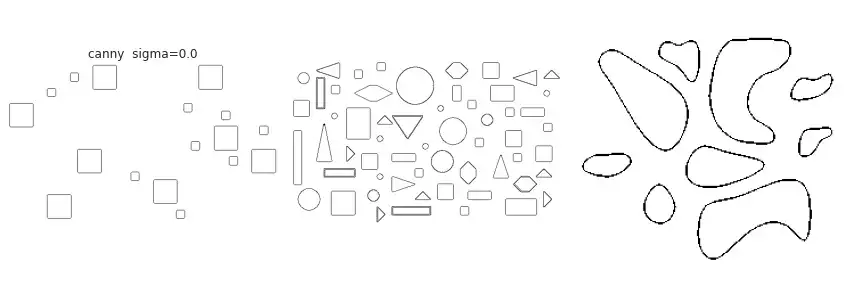

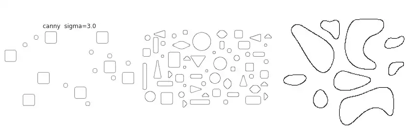
The figure above contains a comparison between the available border extraction methods. Roberts seems to produce the thinnest borders amongst all methods, while Farid produces thicker ones. Sobel, Prewitt and Scharr have similar results. Finally, Canny with a small $\sigma$ parameter (used to set the standard deviation of the Gaussian filter) results in accurate borders for simple shapes. However, the original gray intensity of the object’s border is lost, with all borders presenting the same gray intensity. Canny with a very large sigma parameter ($\sigma=3$) still manages to extract borders from simple objects, though corners become round.
With closed borders in hands, extracted from one of the methods above, we can simply fill the wholes to separate what’s background and foreground:
from scipy import ndimage

segments = [skimage.filters.roberts(g) for g in grays]
filled = [ndimage.binary_fill_holes(s) for s in segments]

visualize(filled, rows=1, cmap='gray_r');
Notice we used the color map gray_r, indicating objects were filled with the value 1 while the background is represented with the value 0.
As each object is now represented by a distinct connected component, we can extract properties using functions in the skimage.measure module:
%%time

from skimage.measure import label
from skimage.measure import regionprops_table

properties = ('label', 'area', 'convex_area', 'eccentricity',
              'solidity', 'perimeter', 'centroid', 'bbox')

segments = [label(f) for f in filled]
props = [pd.DataFrame(regionprops_table(s, properties=properties))
         for s in segments]
CPU times: user 129 ms, sys: 4.74 ms, total: 133 ms
Wall time: 137 ms
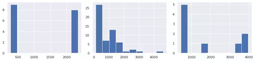
def plot_all_segments(grays, segments, props):
  plt.figure(figsize=(12, 3))
  for ix, (i, s, p) in enumerate(zip(grays, segments, props)):
    plt.subplot(1, 3, ix+1)
    plot_segments(i, s, p)
  plt.tight_layout()

  plt.figure(figsize=(12, 3))
  for ix, (i, s, p) in enumerate(zip(grays, segments, props)):
    plt.subplot(1, 3, ix+1)
    plt.hist(p.area)
  plt.tight_layout()

plot_all_segments(grays, segments, props)
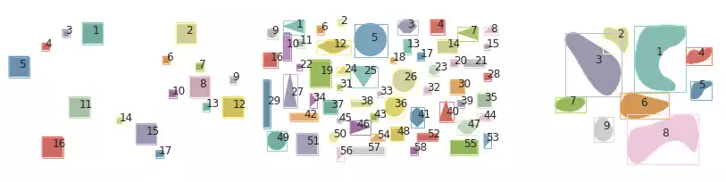
regionprops_table.
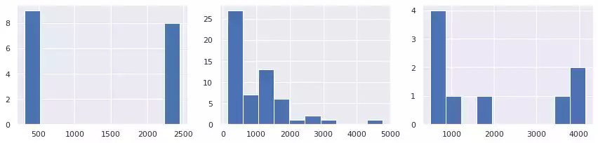
A simple way to count objects based on their overall area is to use histograms. Fig. 5 illustrate this application over each image. In the first, forms are separated into two similar groups: small(close to 500), and large (approx. 2,500). A more diverse set of areas are present in the second image, producing a more disperse histogram. In the last image, three objects have very large area (1, 3 and 8). Object 6 has an intermediate size, while the remaining objects are small.
Segmentation using Felzenszwalb’s Method
This segmentation method was described in “Efficient graph-based image segmentation”, by Felzenszwalb et. al. [3] It consists of representing the pixel-color intensity in an image as a grid and find $N$ partitions representing similarity. As the algorithm progresses, the closest partitions (with respect to a connection predicate) are iteratively merged. The final number of partitions is minimum (optimal) while still respecting the connection predicate.
The following code exemplifies the application of Felzenszwalb’s segmentation method implemented in scikit-image over images:
segments = [skimage.segmentation.felzenszwalb(g, scale=1e6, sigma=0.1, min_size=10) for g in grays]
props = [pd.DataFrame(regionprops_table(s, properties=Config.properties)) for s in segments]

props[0].head().round(2)
| label | area | convex_area | eccentricity | solidity | perimeter | centroid-0 | centroid-1 | bbox-0 | bbox-1 | bbox-2 | bbox-3 | |
|---|---|---|---|---|---|---|---|---|---|---|---|---|
| 0 | 1 | 2352 | 2352 | 0.20 | 1.0 | 190.0 | 29 | 202 | 5 | 179 | 54 | 227 |
| 1 | 2 | 2352 | 2352 | 0.20 | 1.0 | 190.0 | 29 | 422 | 5 | 399 | 54 | 447 |
| 2 | 3 | 272 | 272 | 0.34 | 1.0 | 62.0 | 29 | 139 | 21 | 132 | 38 | 148 |
| 3 | 4 | 272 | 272 | 0.34 | 1.0 | 62.0 | 60 | 92 | 53 | 84 | 69 | 101 |
| 4 | 5 | 2304 | 2304 | 0.00 | 1.0 | 188.0 | 107 | 29 | 84 | 6 | 132 | 54 |
Fig. 6 illustrates the Felzenszwalb’s segmentation results over images containing simple geometric shapes. Little difference can be perceived from the edge-based segmentation strategy.
I used the parameters scale=1e6, sigma=0.1, min_size=10 to detect the simple geometric shapes, which enforces large objects (high scale) and low Gaussian filtering (low sigma). Decreasing scale had little influence in the results of the last sample (containing 9 objects). However, this resulted in an incorrect segmentation for the objects in the first and second images, in which the objects and their borders were being classified as distinct coinciding objects.
I found min_size to be of little importance in these examples, as it is applied as a post-processing stage and can be disregarded when scale is sufficiently large.
plot_all_segments(grays, segments, props)

Similar results are obtained with Felzenszwalb, with respect to the area of objects:
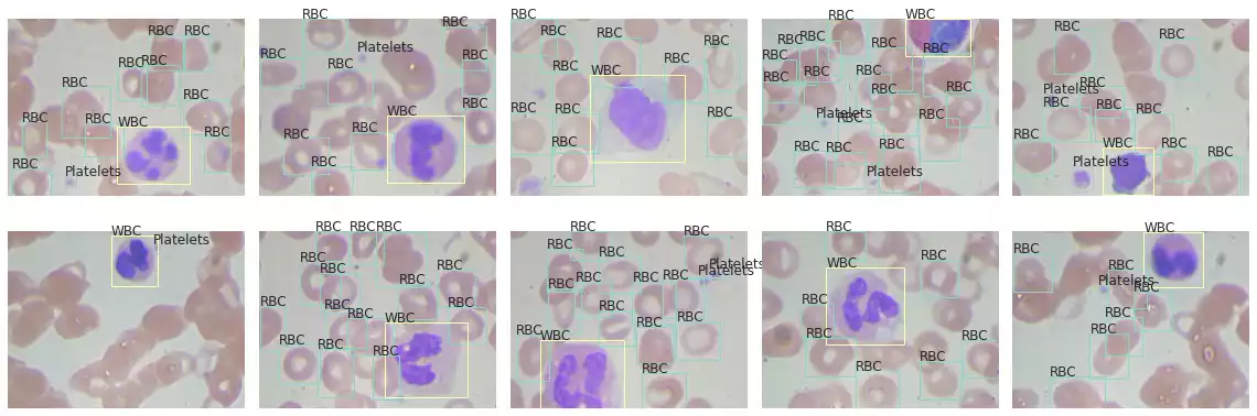
BCCD Dataset
To demonstrate in a more realistic scenario, I opted to use the BCCD Dataset. This set comprises small-scale image samples used for blood cell detection.
import tensorflow as tf
import tensorflow_datasets as tfds

(train,), info = tfds.load('bccd', split=['train'], with_info=True, shuffle_files=False)

int2str = info.features['objects']['label'].int2str

bccd_samples = list(train.take(10))
bccd_images = [s['image'].numpy() for s in bccd_samples]
bccd_grays = [skimage.color.rgb2gray(i) for i in bccd_images]
bccd_cells = sum([e['objects']['label'].shape.as_list() for e in bccd_samples], [])


fig = visualize([s['image'] for s in bccd_samples], rows=2, figsize=(16, 6))
axes = fig.get_axes()

for ax, p in zip(axes, bccd_samples):
    plot_detection_boxes(p, ax)
Segmentation using Felzenszwalb’s Method
Edge-detection methods produce poor results over samples in the BCCD dataset, as they are quite more complex than the ones previously used — presenting salt-and-pepper noise and much more densely distributed objects —. Thus, I once again employed Felzenszwalb’s method.
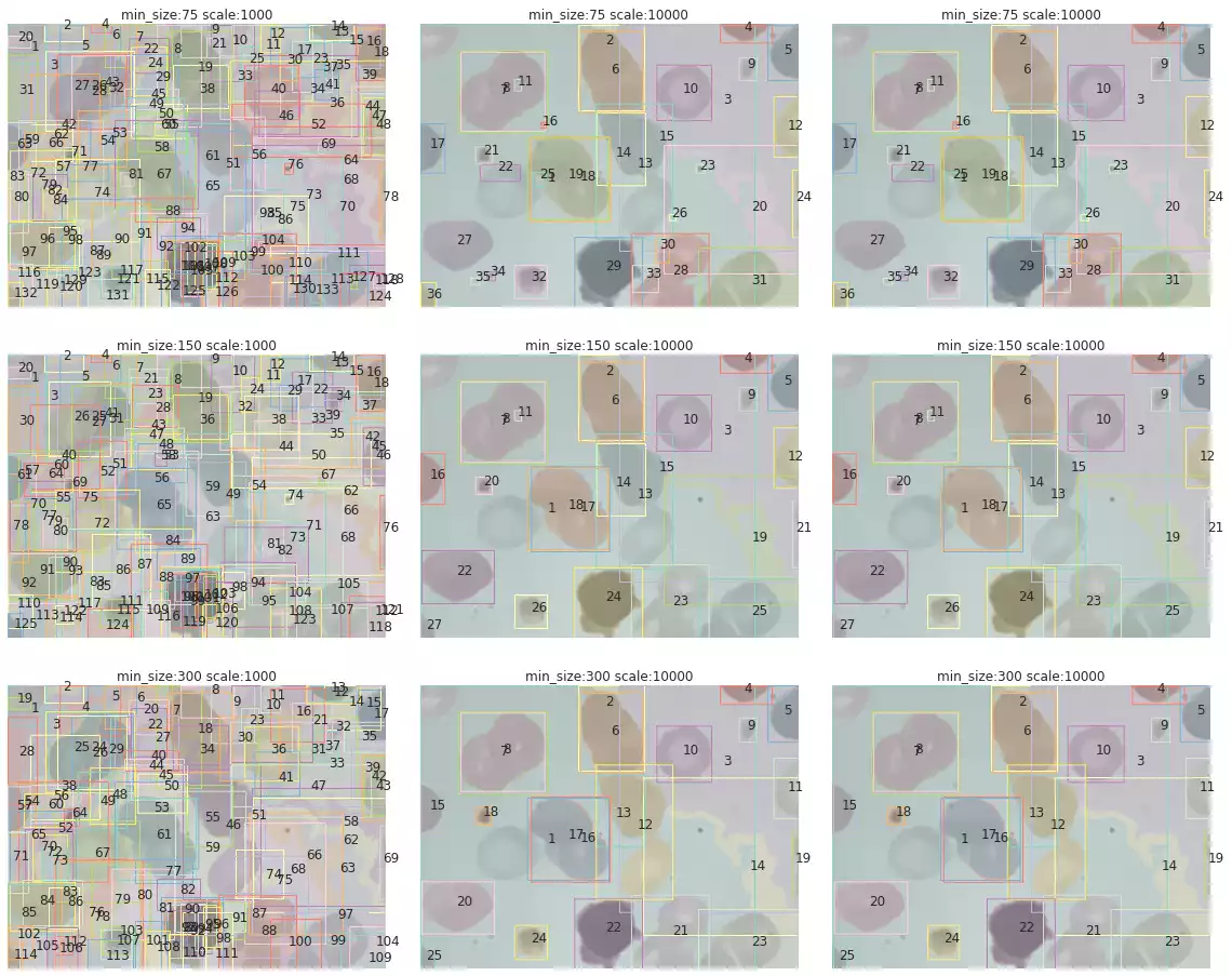
We first “search” for the best combination of parameters to use in this set.
from sklearn.model_selection import ParameterGrid

def search_felzenszwalb(image, params=None, figsize=(16, 13)):
  if not params:
    params = ParameterGrid({
      'scale': [1000, 10000, 10000],
      'min_size': [75, 150, 300],
    })

  plt.figure(figsize=figsize)

  for ix, param in enumerate(params):
    segment = skimage.segmentation.felzenszwalb(image, sigma=0.01, **param)
    prop = pd.DataFrame(regionprops_table(segment, properties=Config.properties))

    ax = plt.subplot(ceil(len(params) / 3), 3, ix+1)
    plot_segments(image, segment, prop, alpha=0.2, ax=ax)
    plt.title(' '.join((':'.join(map(str, e)) for e in param.items())))

  plt.tight_layout()

search_felzenszwalb(bccd_images[3])
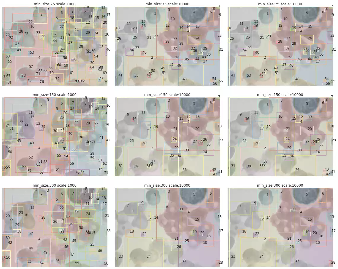
scale and min_size over segmentation.
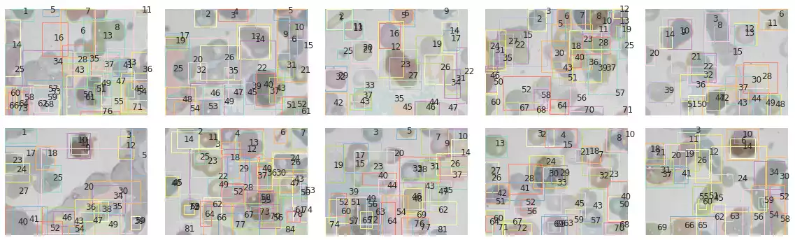
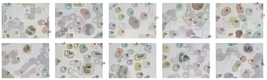
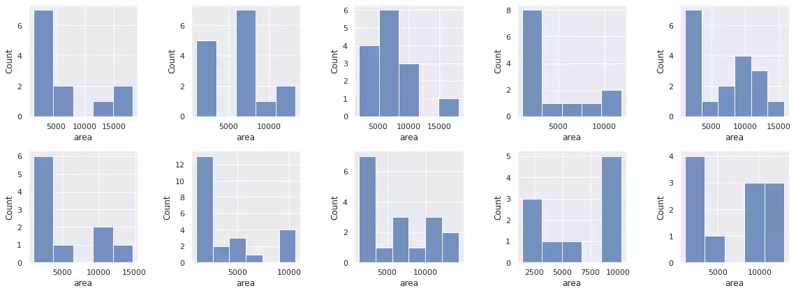
The segmentation results of samples in the BCCD dataset are shown in Fig. 10. The method has correctly segmented many of the blood cells in some samples (such as in the third and fifth images). However, a few drawbacks are noticeable as well: this method is strongly affected by small grains, and will often recognize small microorganisms that were captured by the microscope while photographing the blood cells. Furthermore, cells that were smashed together seem to have been classified as a single object (first and eighth images).
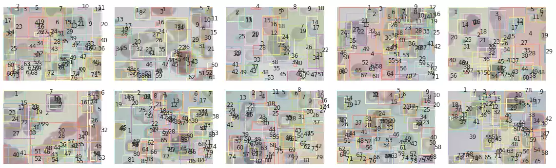
images = bccd_images

segments = [skimage.segmentation.felzenszwalb(i, scale=1e3, sigma=0.01, min_size=150) for i in images]
props = [pd.DataFrame(regionprops_table(s, properties=Config.properties)) for s in segments]
def plot_all_segments_and_bboxes(images, segments, props):
  plt.figure(figsize=(16, 5))

  for ix, (image, label, prop) in enumerate(zip(images, segments, props)):
    ax = plt.subplot(2, 5, ix+1)
    plot_segments(image, label, prop, alpha=0.2, ax=ax)

  plt.tight_layout()

plot_all_segments_and_bboxes(images, segments, props)
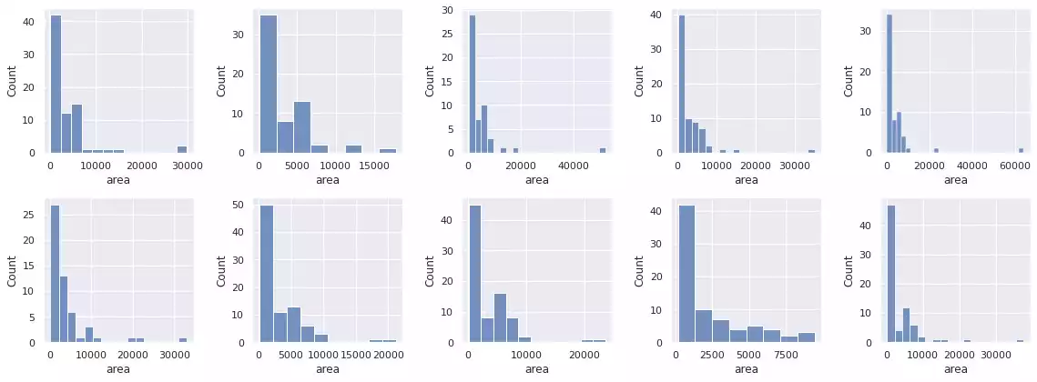
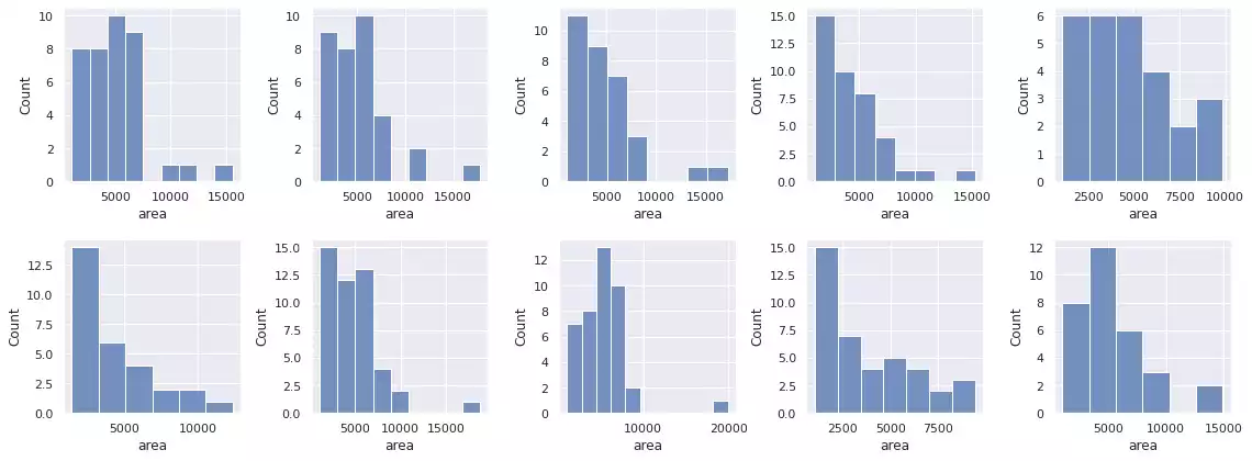
def histogram_objects(props, by='area', percentile=None):
  plt.figure(figsize=(16, 6))

  for ix, prop in enumerate(props):
    plt.subplot(2, ceil(len(props)/2), ix +1)

    s = prop[by]
    if percentile: s = s[s < np.percentile(s, 99)]
    sns.histplot(s)

  plt.tight_layout()

histogram_objects(props, percentile=95)
Finally, Felzenszwalb’s method will indistinguishably segment the background sections of the image into regions, as these sections also present color information. It is therefore necessary to employ heuristics that discriminate foreground/background in order to separate it.
Post-Processing: Filtering Objects by Overall Size
To remedy the grain noise being detected by Felzenszwalb’s, we can sub-select objects based on their properties. A simple selection could be defined by its overall area:
RBC_AREA = (1e3, 2e4)

props_rbc = [p[(p.area > RBC_AREA[0]) & (p.area < RBC_AREA[1])] for p in props]
segments_rbc = [s*np.isin(s, p.label) for s, p in zip(segments, props_rbc)]

plot_all_segments_and_bboxes(images, bccd_samples, segments_rbc, props_rbc)
histogram_objects(props_rbc)
Pre-Processing: Filtering Noise
The noise present in the samples correspond to dirt present in the lab sample, and do not contribute to the detection of blood cells. We can use filters.rank.mean_bilateral to remove this noise before applying segmentation, possibly reducing the complexity and helping Felzenszwalb’s to focus on the cells:
from skimage import color, img_as_ubyte, img_as_float
from skimage.morphology import disk
from skimage.filters.rank import mean_bilateral

selem20 = disk(20)

def mean_bilateral_fn(image, selem, s0=10, s1=10):
  image = color.rgb2gray(image)
  image = img_as_ubyte(image).astype('uint16')
  image = mean_bilateral(image, selem, s0=s0, s1=s1)

  return image / 255.

grays_bilateral = [mean_bilateral_fn(i, selem20) for i in images]

visualize(grays[:5] + grays_bilateral[:5], figsize=(16, 5));
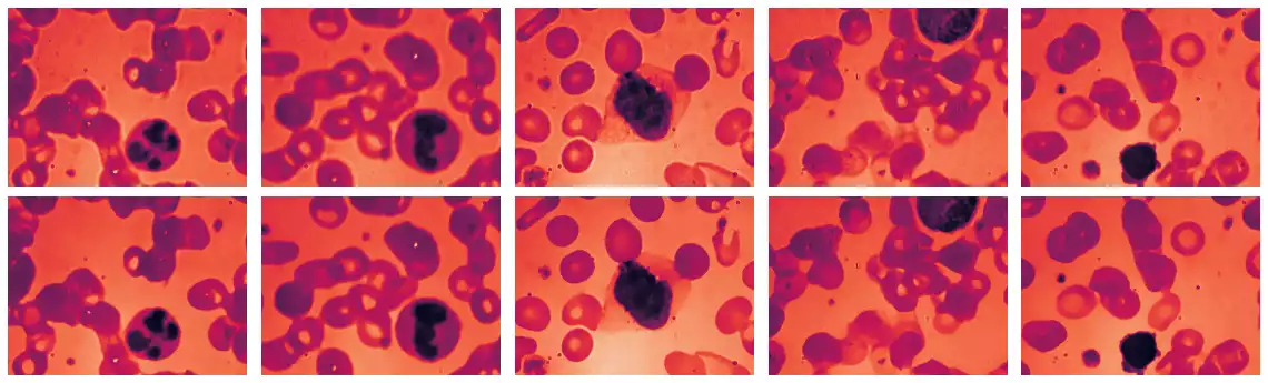
mean_bilateral. From top to bottom: (a) the original samples in the BCCD dataset, (b) the corresponding sample cleaned from noise.
Fig. 14 illustrates the application of mean_bilateral over samples in the BCCD dataset.
We observe that much of the noise is either removed or attenuated.
As samples have changed drastically, we search parameters once again. Fig. 15 illustrates
the effect of varying scale and min_size over a sample in the BCCD dataset. The combination
scale=1e4 and min_size=150 seems to produce reasonable results for this sample.
search_felzenszwalb(grays_bilateral[4])
scale and min_size over segmentation, after preprocessing with mean_bilateral was performed.
We can now apply to each sample in our subset:
# Pre-processing
selem20 = disk(20)
grays_bilateral = [mean_bilateral_fn(i, selem20) for i in images]

# Segmentation
segments = [skimage.segmentation.felzenszwalb(i, scale=1e4, sigma=0.01, min_size=150)
            for i in grays_bilateral]
props = [pd.DataFrame(regionprops_table(s, properties=Config.properties))
         for s in segments]

# Post-processing
RBC_AREA = (1e3, 2e4)

props_rbc = [p[(p.area > RBC_AREA[0]) & (p.area < RBC_AREA[1])] for p in props]
segments_rbc = [s*np.isin(s, p.label) for s, p in zip(segments, props_rbc)]

plot_all_segments_and_bboxes(images, bccd_samples, segments_rbc, props_rbc)
mean_bilateral and post-processing them by sub-selecting objects within a reasonable overall area.
histogram_objects(props_rbc)
From Fig. 16 and Fig. 17 show our cleaned segmentation results. The algorithm seems much more focused on cells now!
Morphological Boundaries
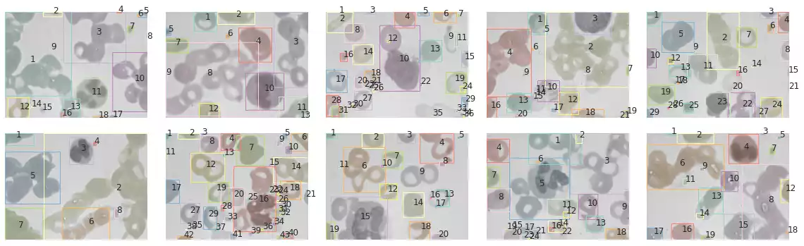
Going in a different direction, morphology can also be used to segment objects in images. I employed a second segmentation strategy, which consists of applying the Ostu’s threshold [2] to separate objects from background and employ morphology to close small holes. The cleaned mask can then be labeled according to its connected regions.
The code below describes the necessary steps to implement this strategy. Notice that the binary mask that will serve as input to the morphological operations is created by retaining the positions in which pixel intensity is below the threshold (image < t), as the objects in this problem present a lower pixel intensity than the background’s. This differs from the examples in scikit-image documentation, in which silver coins were being compared to a dark background.
from skimage.measure import label
from skimage.filters import threshold_otsu
from skimage.morphology import opening, closing, square

def morphological_segmentation(image, so=square(5)):
  bw = image < threshold_otsu(image)

  return label(opening(closing(bw, so),  so))
%%time

images = bccd_grays
segments = [morphological_segmentation(image) for image in images]
props = [pd.DataFrame(regionprops_table(s, properties=Config.properties)) for s in segments]
CPU times: user 1.13 s, sys: 520 ms, total: 1.65 s
Wall time: 1.11 s
plot_all_segments_and_bboxes(images, bccd_samples, segments, props)
histogram_objects(props)
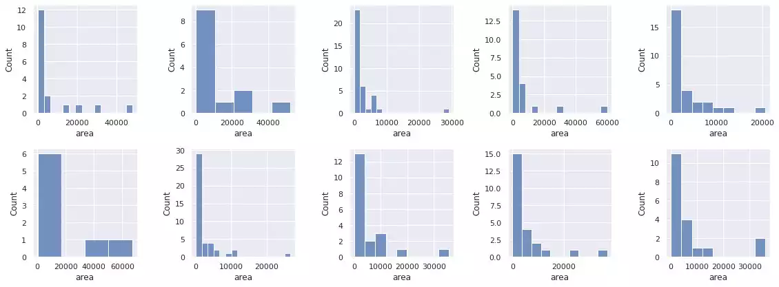
The segmentation results over samples in the BCCD dataset are shown in Fig. 18 and Fig. 19. Through inspection, we notice this strategy is robust against small grains in the image, and correctly segments red blood cells presenting light-shaded interiors. It also automatically ignores the background and does not interpret its regions as new objects — through the usage of Otsu’s method [4] —. Notwithstanding, long cell chains (which are smashed against each other) are incorrectly segmented as a single object, regardless of their color differences (an effect observed in the first, second, third, fifth, ninth and tenth images).
References
- V. Torre and T. A. Poggio, “On Edge Detection,” IEEE Transactions on Pattern Analysis and Machine Intelligence, vol. PAMI-8, no. 2, pp. 147–163, 1986, doi: 10.1109/TPAMI.1986.4767769.
- A. N. Strahler, “Quantitative analysis of watershed geomorphology,” Eos, Transactions American Geophysical Union, vol. 38, no. 6, pp. 913–920, 1957.
- P. F. Felzenszwalb and D. P. Huttenlocher, “Efficient Graph-Based Image Segmentation,” International Journal of Computer Vision, vol. 59, no. 2, pp. 167–181, Sep. 2004, doi: 10.1023/B:VISI.0000022288.19776.77.
- N. Otsu, “A Threshold Selection Method from Gray-Level Histograms,” IEEE Transactions on Systems, Man, and Cybernetics, vol. 9, no. 1, pp. 62–66, 1979, doi: 10.1109/TSMC.1979.4310076.